Theoretical profiles and fitting from models – CRYSOL in RAW
One of the most useful things to do with SAXS data is to compare the data against high resolution models (such as crystallography or CryoEM structures or AlphaFold models). You can generate theoretical scattering profiles from high resolution models, such as pdb models, independent of the experimental data. You can also fit these generated theoretical scattering profiles against the experimental SAXS data.
While it might seem that the most rigorous approach would be to generate a theoretical profile independent of the experimental data, this ‘minimal’ approach often fails to produce good fits even when the model and solution structure are in good agreement. This is because there are contributions from the solvent, particularly the hydration layer and the excluded volume, that are hard to model and that most theoretical scattering profile calculators treat as fit parameters. So to get the most accurate understanding of whether your model fits the data, you should actually fit the data as part of the process of generating the theoretical profile, rather than generating a ‘minimal’ theoretical profile and comparing to the data.
One of the most common programs to generate theoretical scattering profiles is the CRYSOL program in the ATSAS package. We will use RAW to run CRYSOL. Note that you need ATSAS installed to do this part of the tutorial.
If you use RAW to run CRYSOL, in addition to citing the RAW paper, please cite the paper given in the CRYSOL manual.
The written version of the tutorial follows.
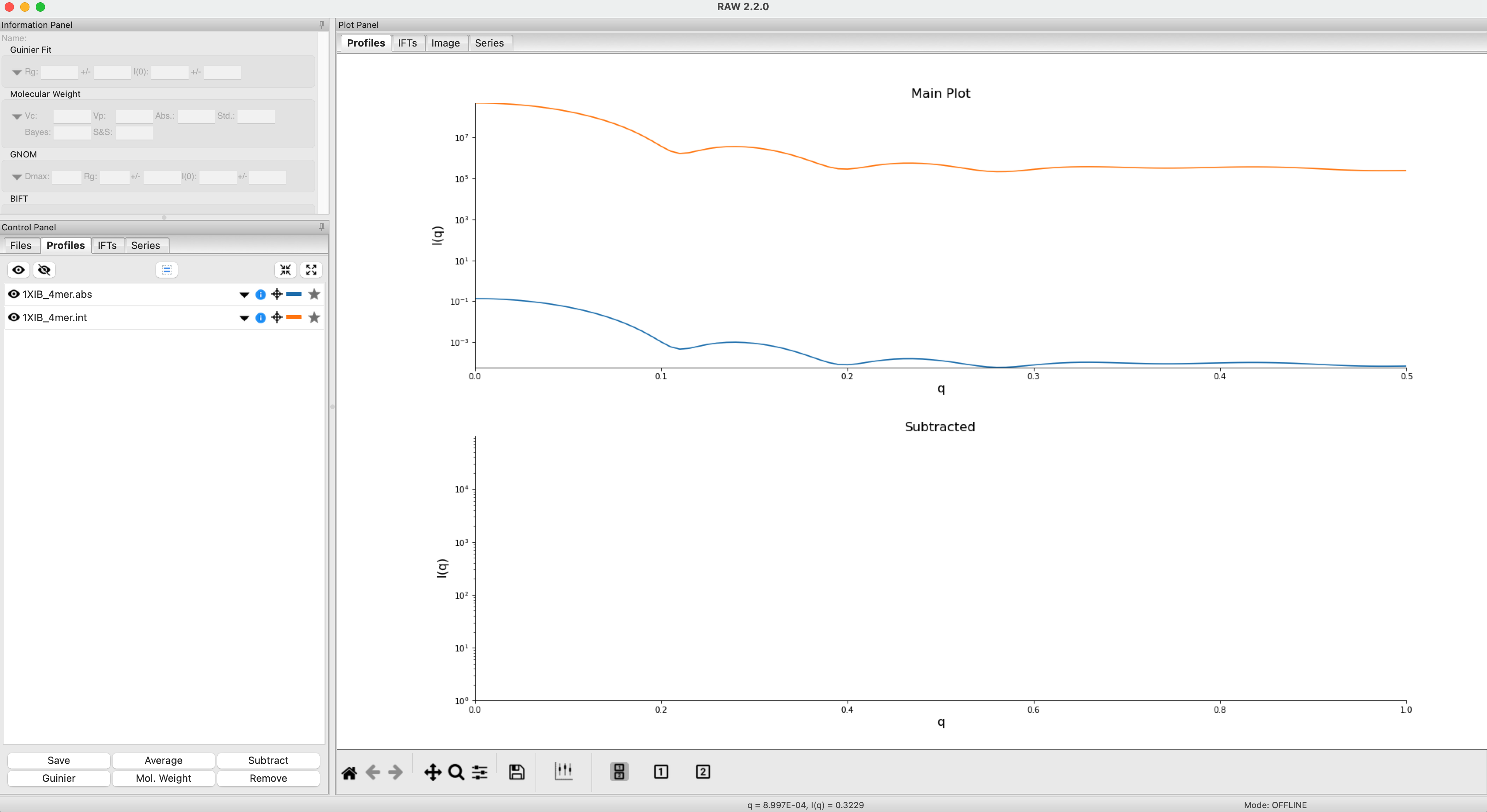
The easiest way to generate a theoretical profile in RAW using CRYSOL is simply to plot a .pdb or .cif file. In the Files Control Panel go to the theory_data folder, select the 1XIB_4mer.pdb and click the plot button.
After the calculation is done, RAW will plot the theoretical profiles from CRYSOL on the profiles plot. You should see two profiles, 1XIB_4mer.abs and 1XIB_4mer.int
Note: The difference between .abs and .int results from CRYSOL is simply the overall scale factor. The .abs is on an absolute scale of 1/(cm*(mg/ml)), while .int is on an arbitrary scale. Generally .abs is probably more useful, since many beamlines calibrate their experimental data to an absolute scale, so this result will be relatively close in overall scale to what you measure.
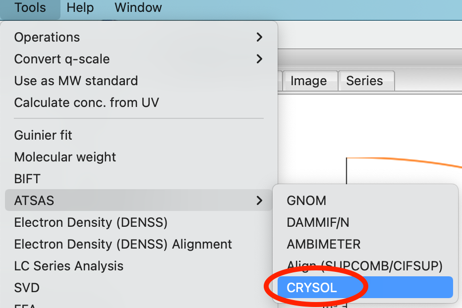
You can also generate a theoretical profile using the CRYSOL window in RAW. This gives you more control over the parameters used to generate the profile, using the plot button simply uses the default parameters. Select the “Tools->ATSAS->CRYSOL” menu option to open the CRYSOL window.
In the CRYSOL window, in the models section use the Add button to add the 1XIB_4mer.pdb file to the list of models to calculate a theoretical profile from.
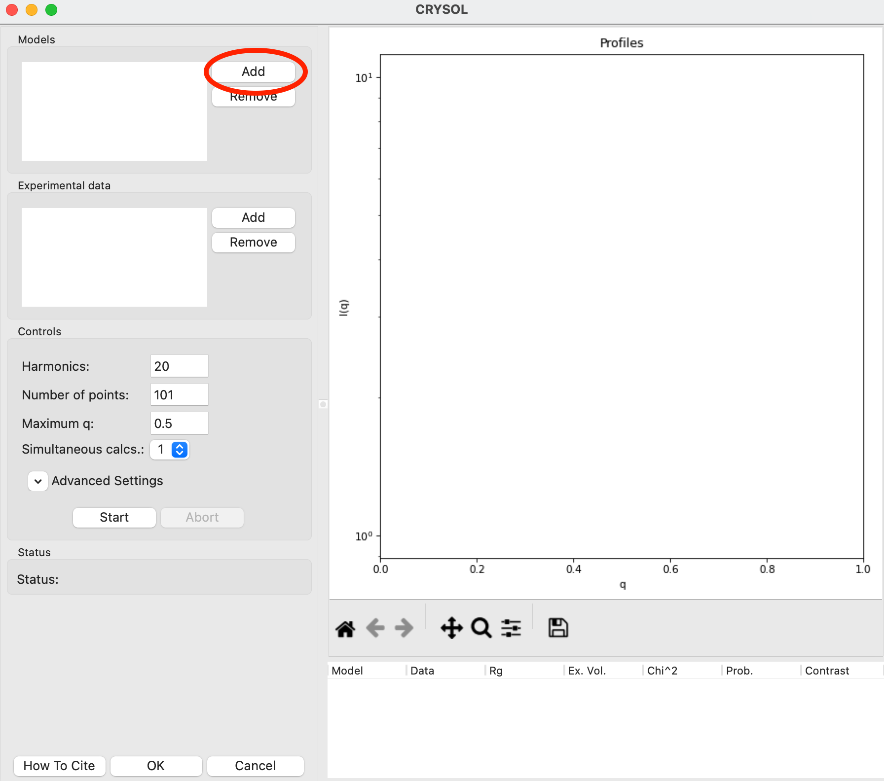
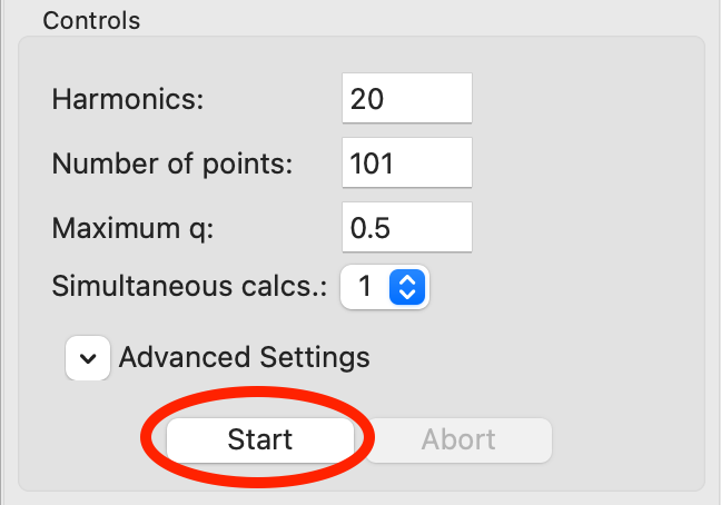
Click the “Start” button to calculate the theoretical scattering profile for the model.
Note: The Status will change to “Running calculation” while running and then to “Finished calculation” when finished.
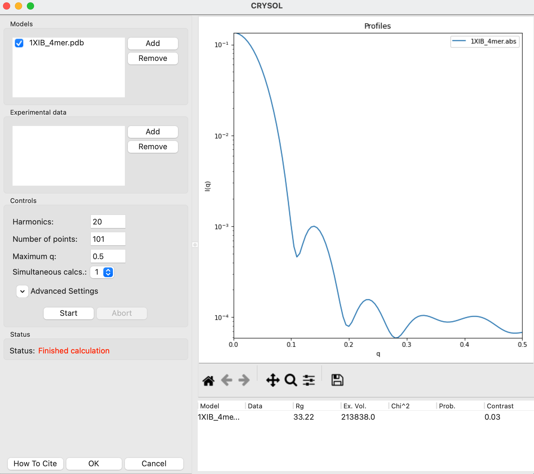
After the calculation finishes, the theoretical profile will display in the plot on the right side of the window, and parameters from the profile will be shown in the list at the bottom right of the window.
Note: Not all parameters will display. The Data, Chi^2, and Prob. fields are only calculated if the model is fit to data.
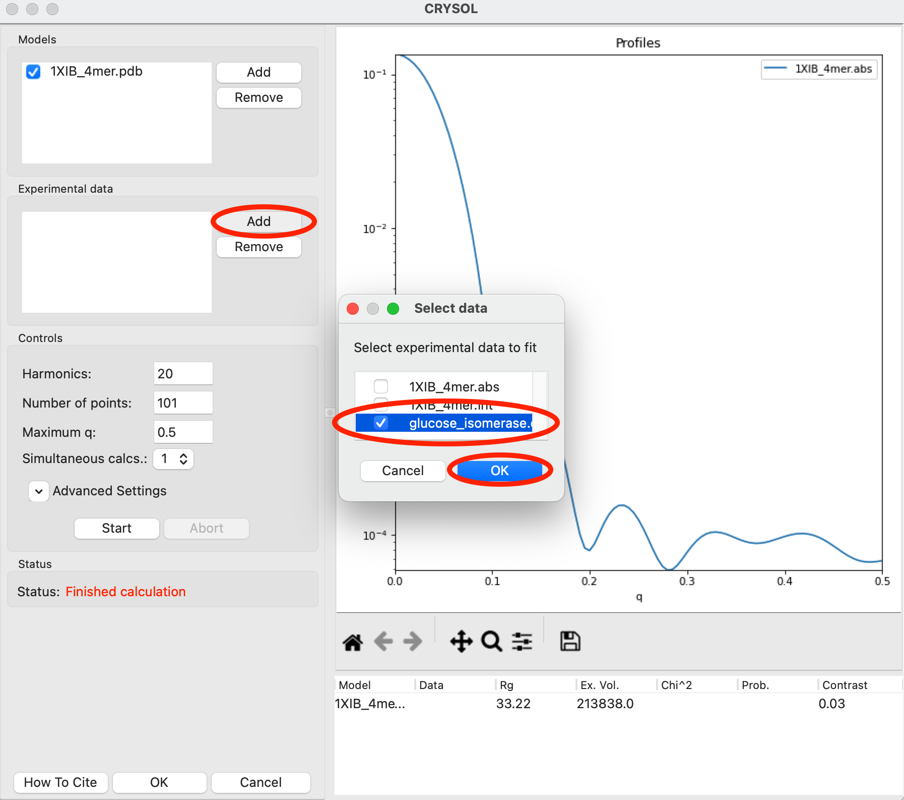
The CRYSOL window can also be used to fit the model against experimental data. Go back to the Files Control Panel and load in the glucose_isomerase.dat data. Return to the CRYSOL window. In the Experimental data section use the Add button, check the glocuse_isomerase.dat item in the dialog that appears, and then click OK to add the glucose_isomerase.dat experimental data to the list of data you can fit a model against.
Note: Only data that is loaded into RAW can be added to the CRYSOL experimental data list.
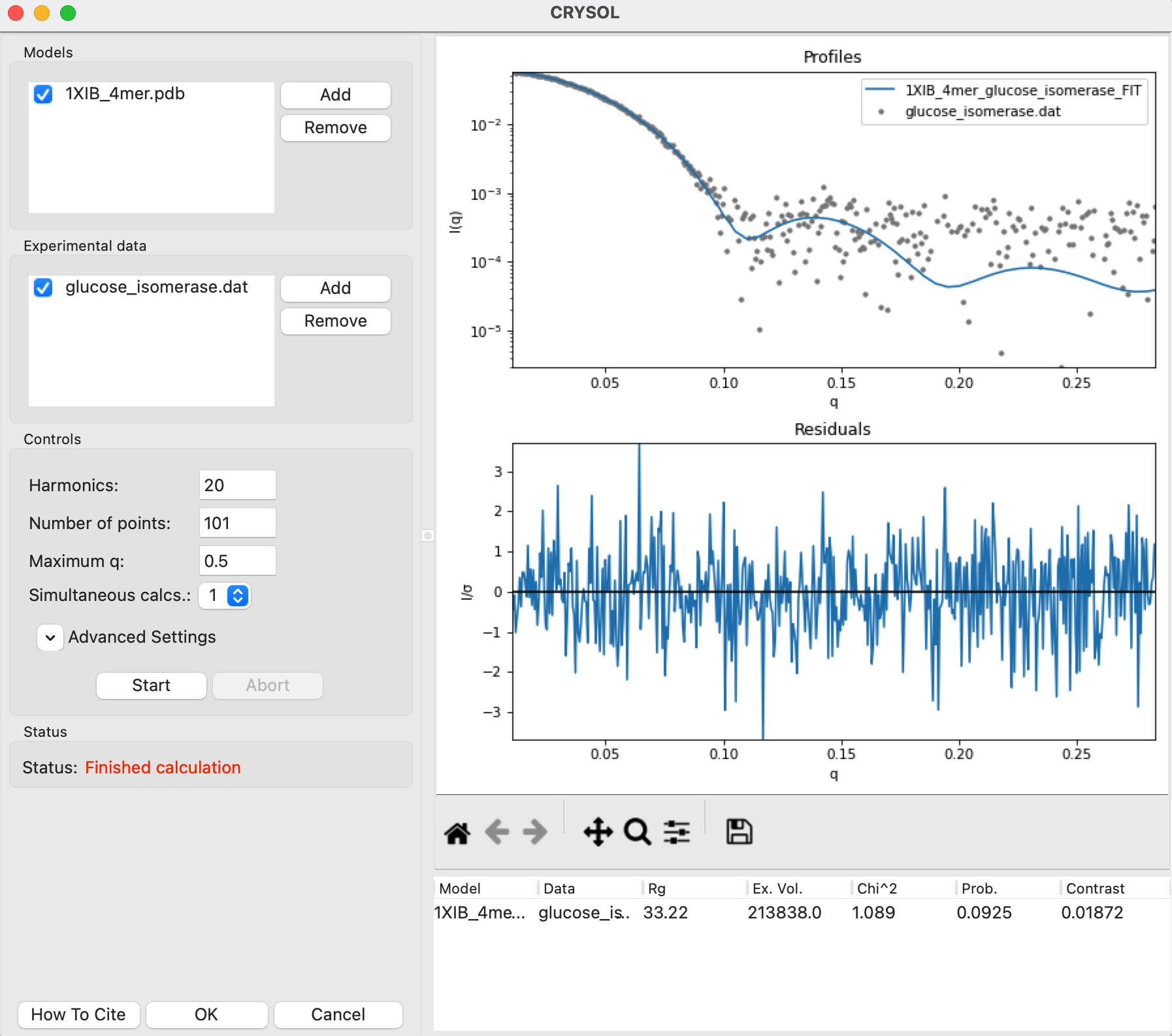
Click the Start button to calculate the theoretical scattering profile and fit it to the data. After the calculation finishes you’ll see both the theoretical profile, the data, and the uncertainty normalized residual plotted in the right plot, as well as the parameters from the theoretical profile in the list at the bottom right.
Note: This will now have all parameters, including the Data, Chi^2, and Prob. fields that were missing when you calculated a theoretical profile without fitting.
Click the OK button to close the CRYSOL window and send the calculated theoretical scattering profile to the Profiles plot. It will appear as 1XIB_4mer_glucose_isomerase_FIT in the Profiles Control Panel.
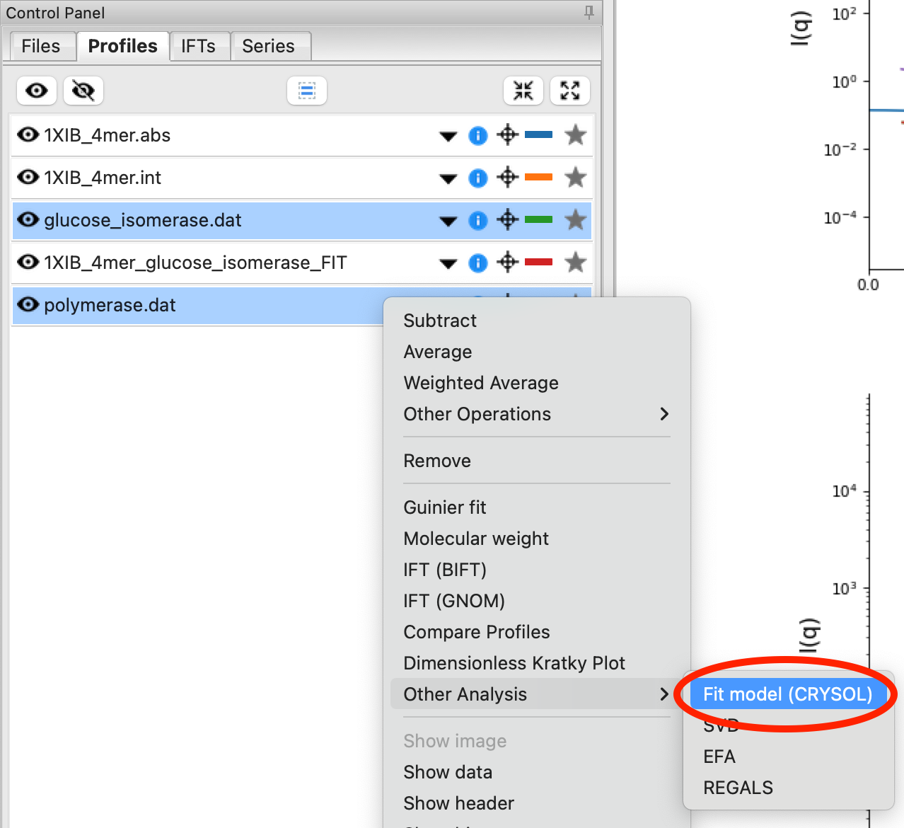
You can also load more than one model and/or profile into the CRYSOL window to calculate multiple profiles at once. Load the polymerase.dat experimental data into RAW. Select both the polymerase and GI profiles in the Profiles Control Panel, right click on the polymerase.dat profile and select “Other Analysis->Fit Model (CRYSOL)”. This will open the CRYSOL window with the selected profiles already loaded in the Experimental Data section.
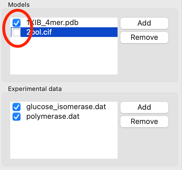
Add the 1XIB_4mer.pdb (GI) and 2pol.cif (polymerase) models to the CRYSOL model section.
Uncheck the 2pol.pdb model in the Models list. Only items that are checked are used for calculation, so this will let you fit just the 1XIB_4mer.cif model.
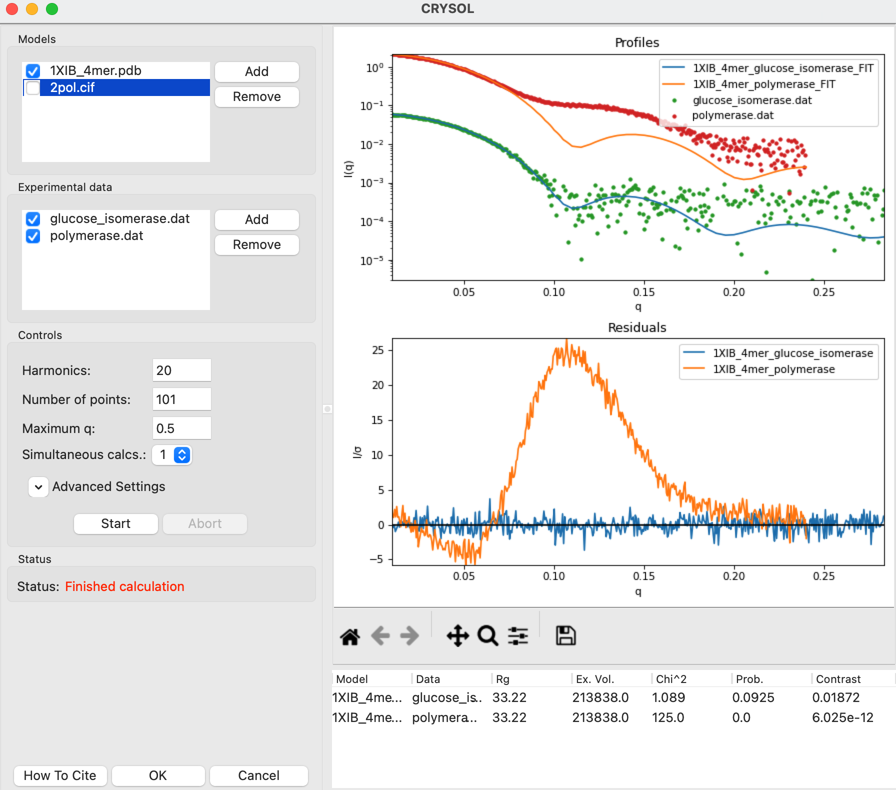
Click the Start button to fit the 1XIB_4mer.cif model against both experimental profiles. After the calculation finishes you’ll see both experimental profiles and the theoretical profile fit to both measured profiles.
Question: Which dataset does the model fit better?
Try: Turn off the 1XIB_4mer model and turn on the 2pol model and see how that fits both profiles.
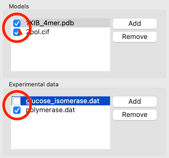
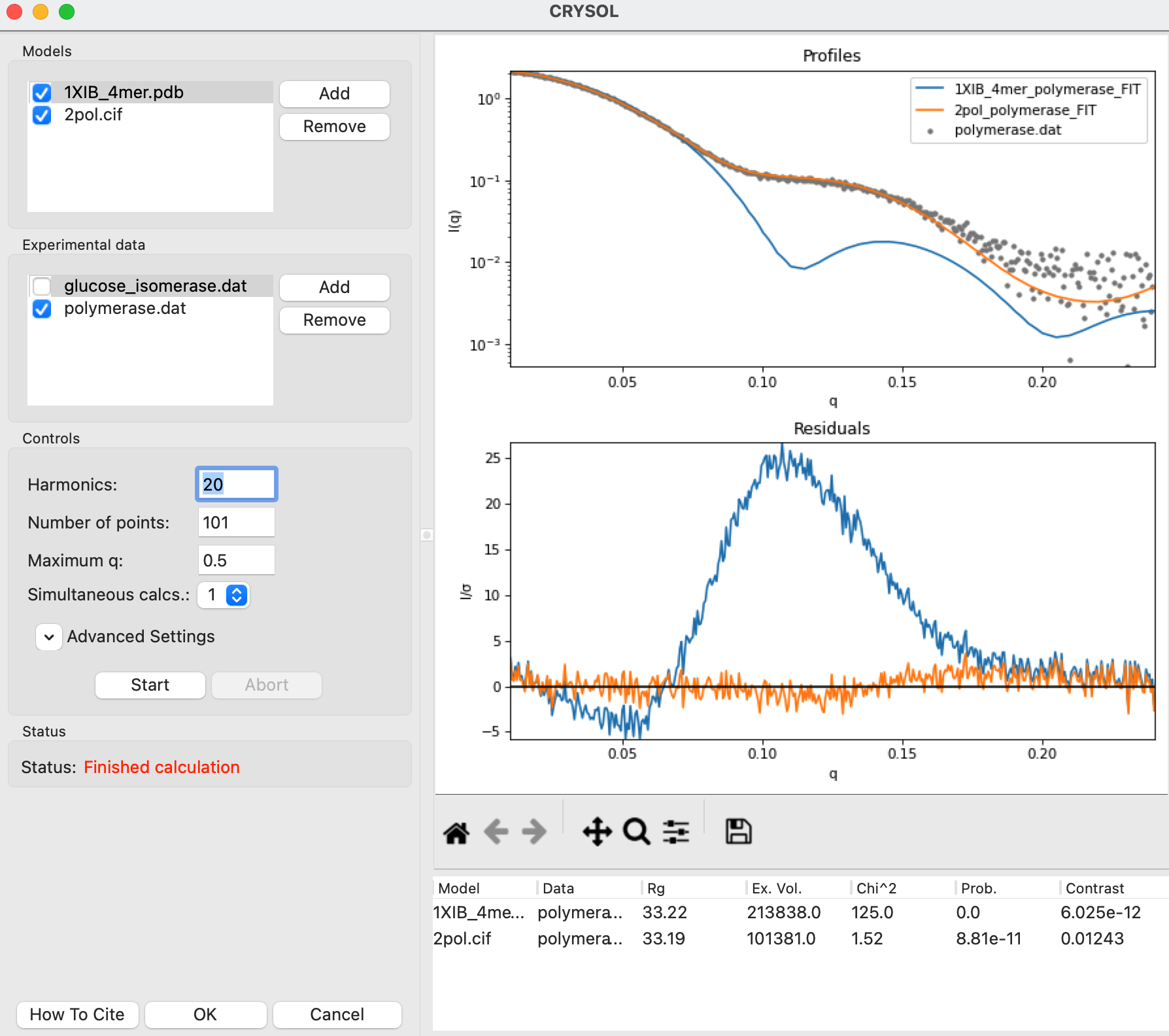
You can also fit multiple models against a single profile. Check both the 1XIB_4mer.pdb and 2pol.cif entries in the models list and uncheck the glucose_isomerase.dat experimental data.
Click the Start button to fit both models against the polymerase data.
Question: Which model fits the profile better?
Try: Turn off the polymerase profile and turn on the GI profile and see how each model fits that data.
Tip: You can also calculate the theoretical scattering profile from multiple models without fitting against data. To do this, uncheck all the data items and calculate the ‘minimal’ theoretical profiles.
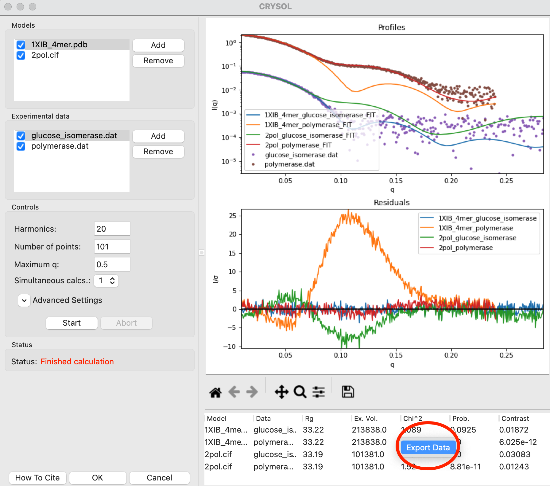
You can fit multiple models against multiple profiles. Check both models and both experimental profiles. Click the start button to fit both models against both experimental profiles.
You can export the values in the results table to a csv file. Right click on the table and select Export Data. Save the .csv file in the theory_data folder.
Try: Open the .csv file in Excel or another spreadsheet program.
Click OK to close the CRYSOL window and send all the fits to the Profiles plot and control panel.
You can also adjust the settings for running CRYSOL from the CRYSOL window. We’ll do that using some example data. Load the SASDP43.dat experimental data into RAW.
Note: This dataset is from the SASDP43 entry in the SASBDB
Open a CRYSOL window and add the Brpt55_M_Zn.pdb model and the SASDP43.dat data.
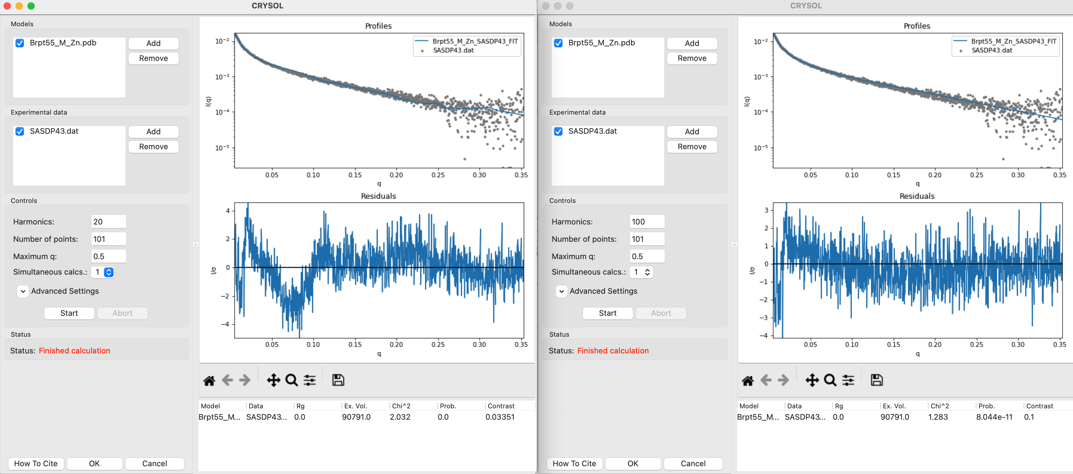
Run the CRYSOL fitting with the default settings.
Open a second CRYSOL window and add the same model and data to it. Set the harmonics to 100. Run the CRYSOL fitting with these updated settings.
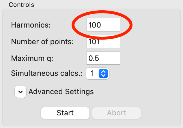
You should see that the result using 100 harmonics is a better fit than the result using the default harmonics.
Note: More harmonics are necessary to get accurate theoretical profiles from high aspect ratio objects. This protein happens to be a long thin rod, so using more harmonics is helpful here. For something globular, like GI, it should make little or no difference. You can test this yourself using the tutorial data.
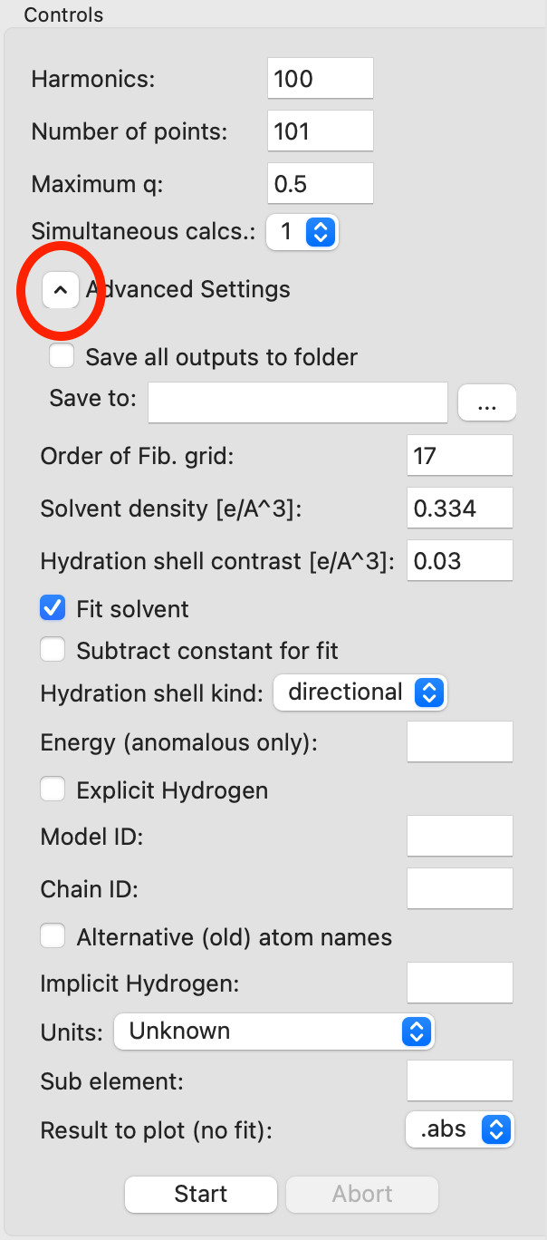
There are also a number of advanced settings you can set. Expand the Advanced Setting section and (if necessary) scroll down to see the different options. The settings are explained in detail in the CRYSOL manual.
Note: Common settings to change are the solvent density and contrast (requires turning off the “Fit solvent” option).
Tip: If you need all the CRYSOL outputs (such as the .log and .alm files) you can check the “Save all outputs to folder” option and provide a folder to save to by clicking the “…” button after the “Save to” field.
Close the CRYSOL windows with the OK button to save the fit results to the Profiles plot and control panel.
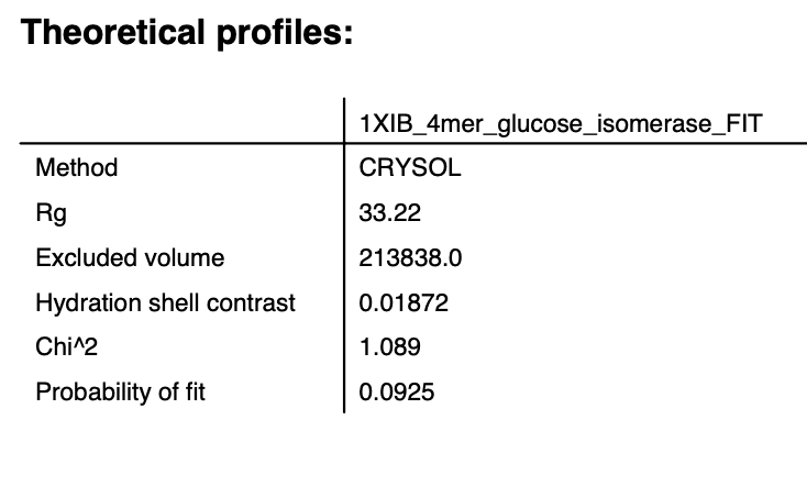
You can save information from a theoretical profile generated by CRYSOL in RAW as part of a pdf report. Right click on the 1XIB_4mer_glucose_isomerase_FIT item in the Profiles control panel and select “Save report”. In the window that opens click “Save Report” and save the pdf report. If you open the report you will see the usually summary pots and a table with a summary of theoretical profile parameters.