Centering and calibration
The next step is to set the beam center, x-ray wavelength, and sample to detector distance. Before this can be done, you have to set the image and file header type in the Options window. The best way to find the beam center and sample to detector distance is using the automated method in RAW. This tutorial assumes you have just done Part 1. If not, open RAW as in Step 1 and set your data folder as in Step 8 of Part 1.
A video version of this tutorial is available:
The written version of the tutorial follows.
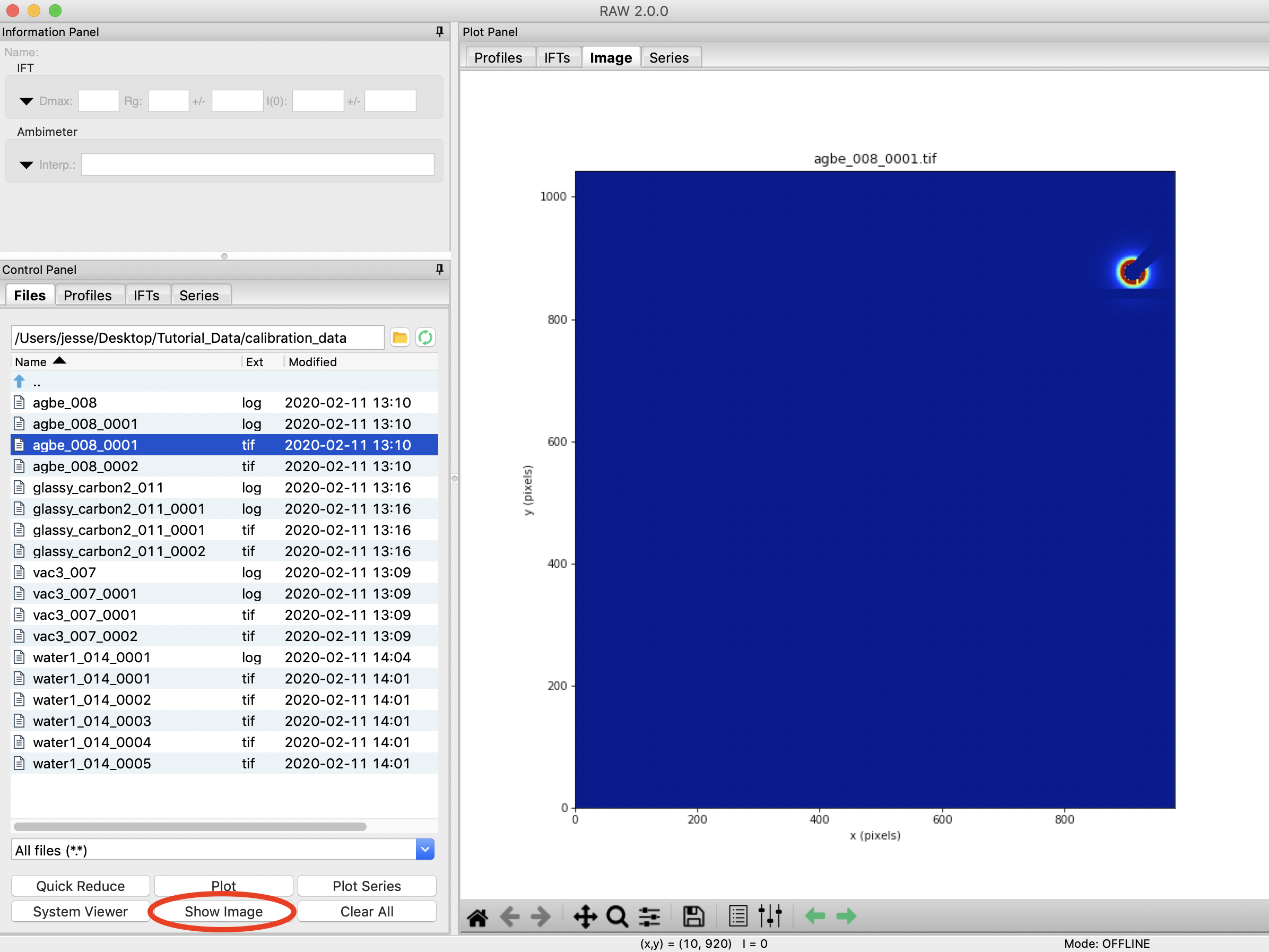
We will use silver behenate to calibrate the sample to detector distance, the beam center on the detector, and the detector rotation. Show the silver behenate image by selecting the agbe_008_0001.tif file and clicking the show image button at the bottom of the File Control panel.
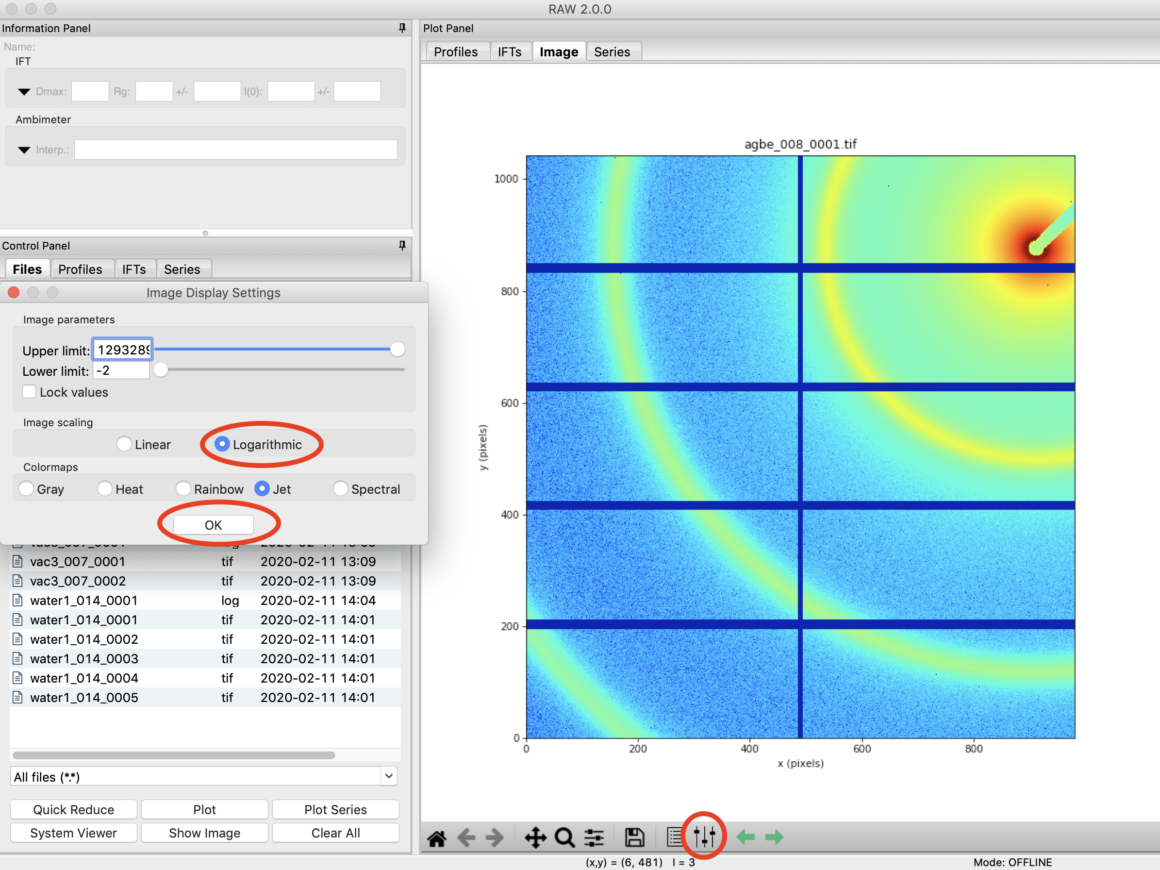
In the Image Plot Panel that is now showing, click on the Image Display Settings button (looks like vertical slider bars) at the bottom of the screen.
In the window that appears, set the scale to logarithmic and and click “OK”.
Open the Centering/Calibration panel by going to the Tools menu and selecting “Centering/Calibration”.
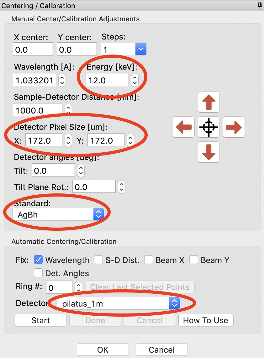
In the Centering/Calibration panel set the Energy to 12.0 keV. Verify that the Detector Pixel Size is 172.0 x 172.0 micron. Verify that the Detector is set to “pilatus_1m”. Verify that the standard is set to AgBh.
Note: The x-ray energy/wavelength is a previously measured value.
Note: If you set the detector properly in the radially averaging options panel the detector and detector pixel size values will fill in automatically (if the detector is not Other).
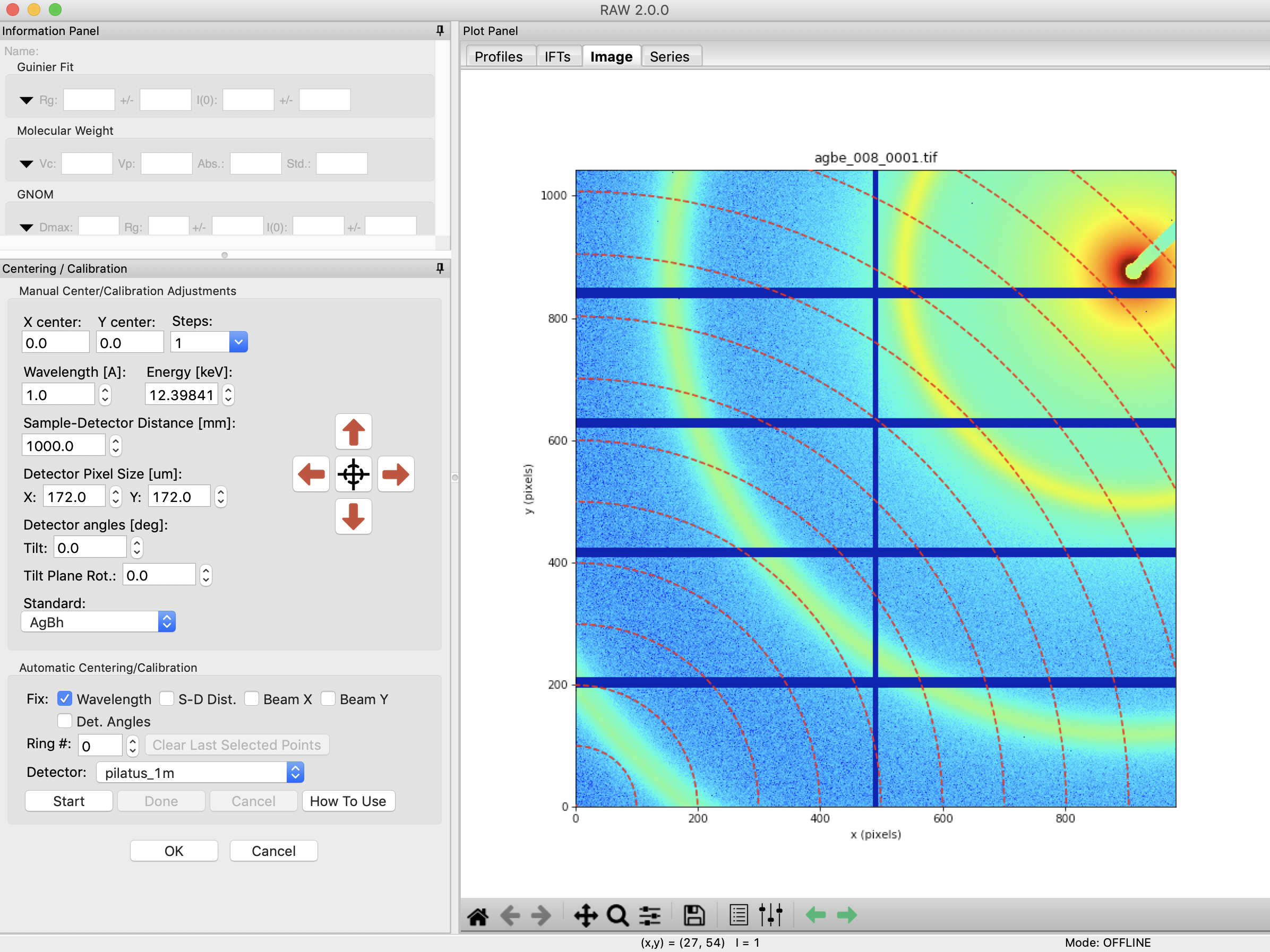
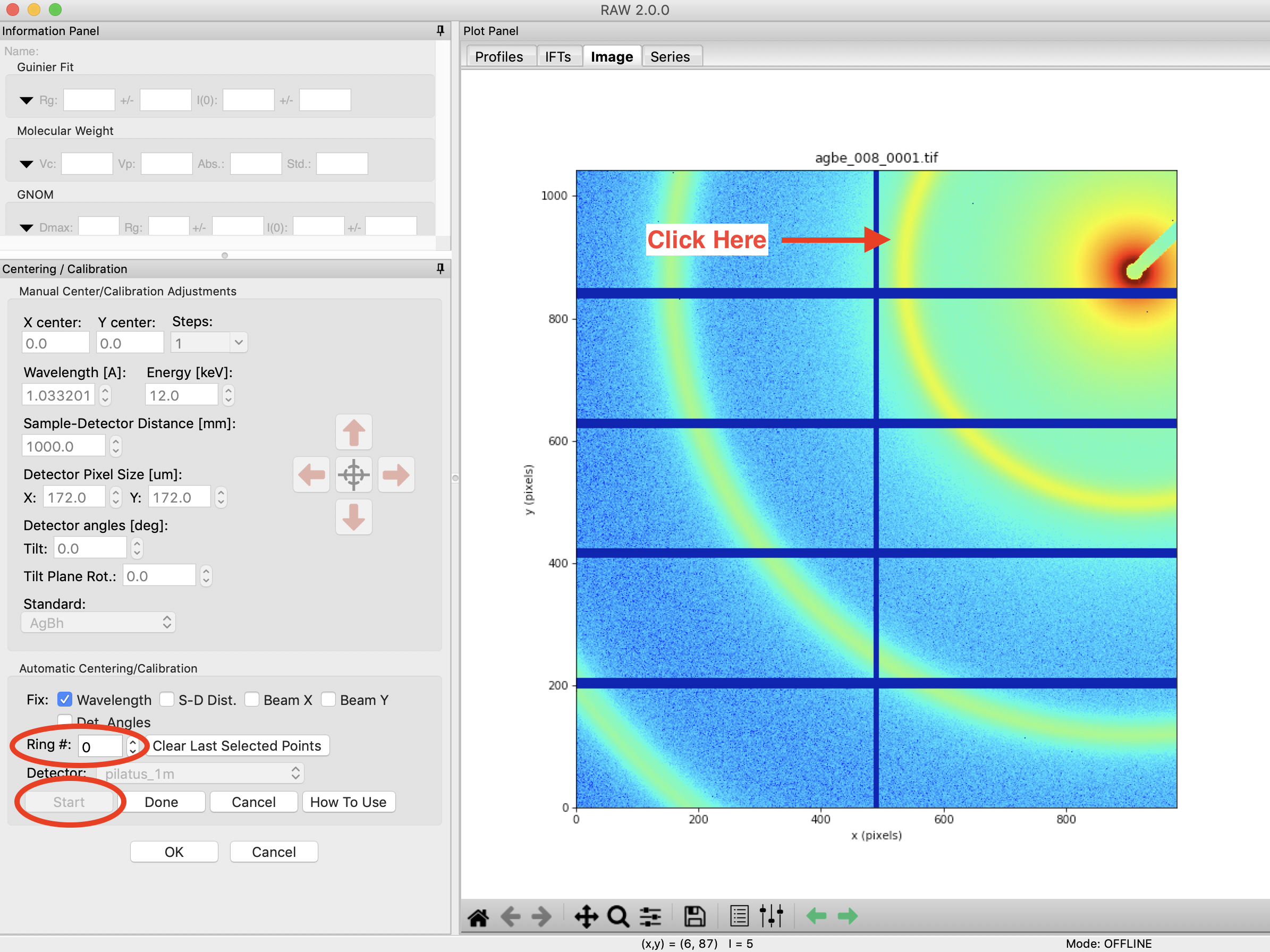
The goal of centering and calibration is to find a beam center position, sample to detector distance, and detector rotation that causes the calculated Silver Behenate ring pattern to match up with the rings on the image.
Note: The beamstop is the blue/green bar extending out from the top right edge of the detector
Click the “Start” button in the “Automatic Centering/Calibration” panel.
Make sure the “Ring #” is set to 0. Click on a point with strong intensity in the Silver Behenate ring nearest the beamstop.
Note: For some experimental setups, one or more of the largest d-spacing rings may not be visible on the detector. In this case, you need to figure out what the first visible ring on the detector is, and set the ring number to that. So, if the third ring was the first one on the detector, the Ring # would be set to 2 (the ring number is zero index, so 0 corresponds to the first ring, 1 to the second ring, and so on).
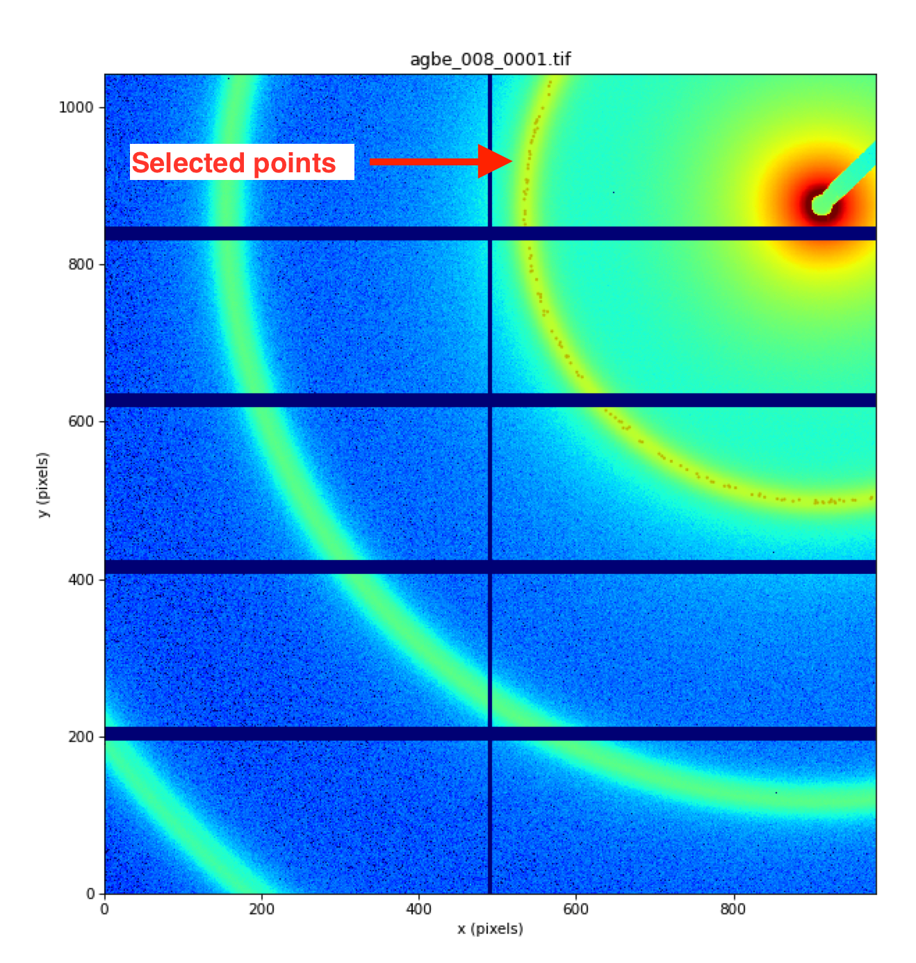
The peak intensity points in that ring will be automatically found, and labeled with tan-ish dots.
Tip: If it didn’t find very many points, try clicking again on another part of the ring, and it will add more points to your selection.
If needed, click on the other portions of the same ring that are on different detector panels to find out the rest of the points in this calibration ring.
Note: The autofind algorithm will only find peaks in contiguous regions. However, masked regions don’t count, so if you’ve masked the panel gaps before calibration it should find points in all of the panels.
Tip: Due to the color map selected, the points may be hard to see. Try changing to the heat map or grayscale to see the selected points,.
Change the “Ring #” to 1.
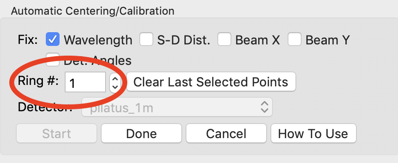
Click on a peak intensity point of the second visible ring. Do this for all the sections of this ring in different detector modules.
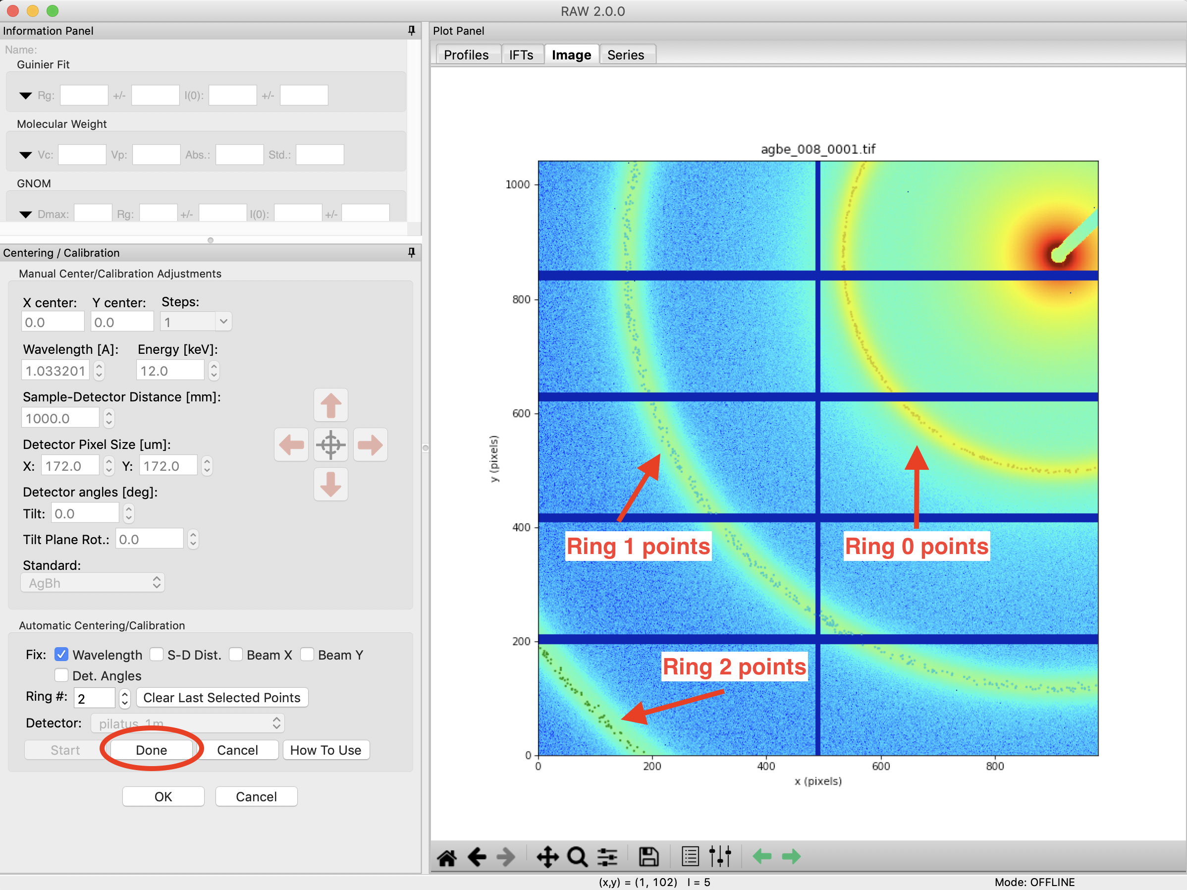
Change the “Ring #” to 2. Click on a peak intensity point of the third visible ring. Points will be shown with green dots.
Click the “Done” button in the “Automatic Centering/Calibration” panel.
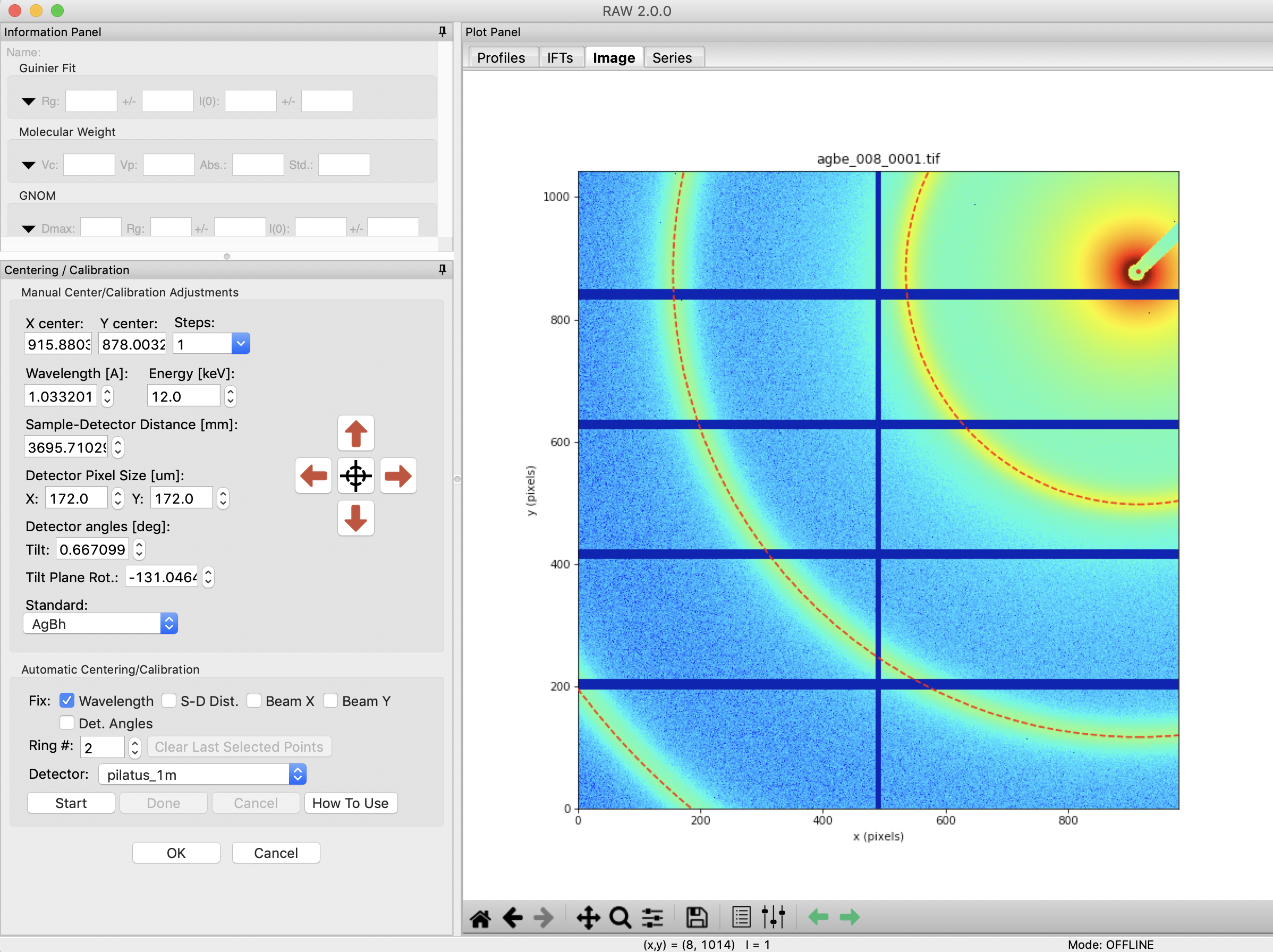
The beam position, sample to detector distance, and detector tilt angles will be calculated and filled in. Calculated rings will display on the plot as dashed red lines, based on the parameters found in the fit. The beam center is displayed as a red dot on the image. You can verify the validity of the fit based on how these calculated values match up with what is shown on the image.
Note: Calculated rings are displayed without detector tilt angles, so if the detector is significantly off beam normal the calculated rings will not match up with the measured rings.
Note: Image tilt plane rotation is an odd value. It represents motions of both X and Y around the Z axis of the detector. As such, it can take on large values (such as -131) for very small detector angles, which is just representing motion in both axes. In this case, all three detector angles are ~0.7 degrees or less.
If necessary (such as if the autocentering routine fails), all of the calibration values can be adjusted manually. The beam center can either be typed into the appropriate boxes, or the red arrows can be used to nudge it by “Steps” pixels in any direction. The crosshairs can be used to pick the beam center position by hand, good for getting a rough alignment. The other parameters can be typed into their appropriate boxes. Manual centering is an iterative process:
Enter rough values based on observation, measurement of actual sample detector distance.
Use arrows to move beam center until you match up with the first ring.
Adjust the distance until you match up with the second ring.
Repeat the last two steps as necessary until you converge on a solution.
Click the OK button in the Centering/Calibration panel to save your settings and exit the panel.