Setting absolute scale with glassy carbon

This section teaches you how to set up absolute scale using glassy carbon (NIST SRM 3600) as a reference. It assumes you have completed Parts 1 (or 2), 3 and 4. Note that you can use water (Part 5) or glassy carbon for absolute scale calibration in RAW.

There are two ways to use glassy carbon as a standard in RAW. One way follows the NIST protocol, and will deliver the most accurate results. However, this method depends on all measurements having reliable flux measurements upstream and downstream of the sample. It also requires accurate measurements of the background of the glassy carbon measurement and the sample measurements. The second way is more similar to that used by water, in that it essentially ignores the background (assumes it to be small). This approach only requires regular normalization and a single measurement of the background for the glassy carbon sample.

The simple approach, “ignoring” background:

1. Load/use the settings from part 4 (without absolute scale set from water, part 5).

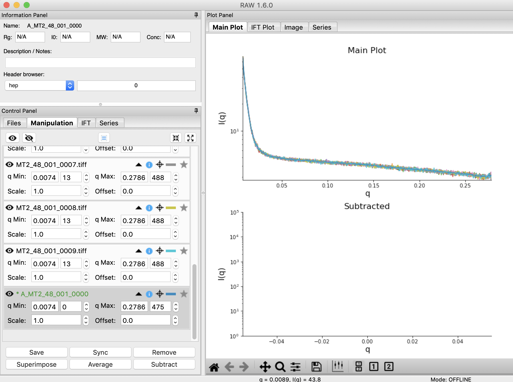
2. Plot all of the glassy_carbon_41_001_000x.tiff files, where x is 0-9, on the main plot.

   • Tip: Section 1 Part 1 of this tutorial document teaches you how to do this.

3. Average the glassy_carbon files you just loaded. Save the average in the calibration_data folder.

4. Open the Options window by selecting “Advanced Options” in the Options menu.

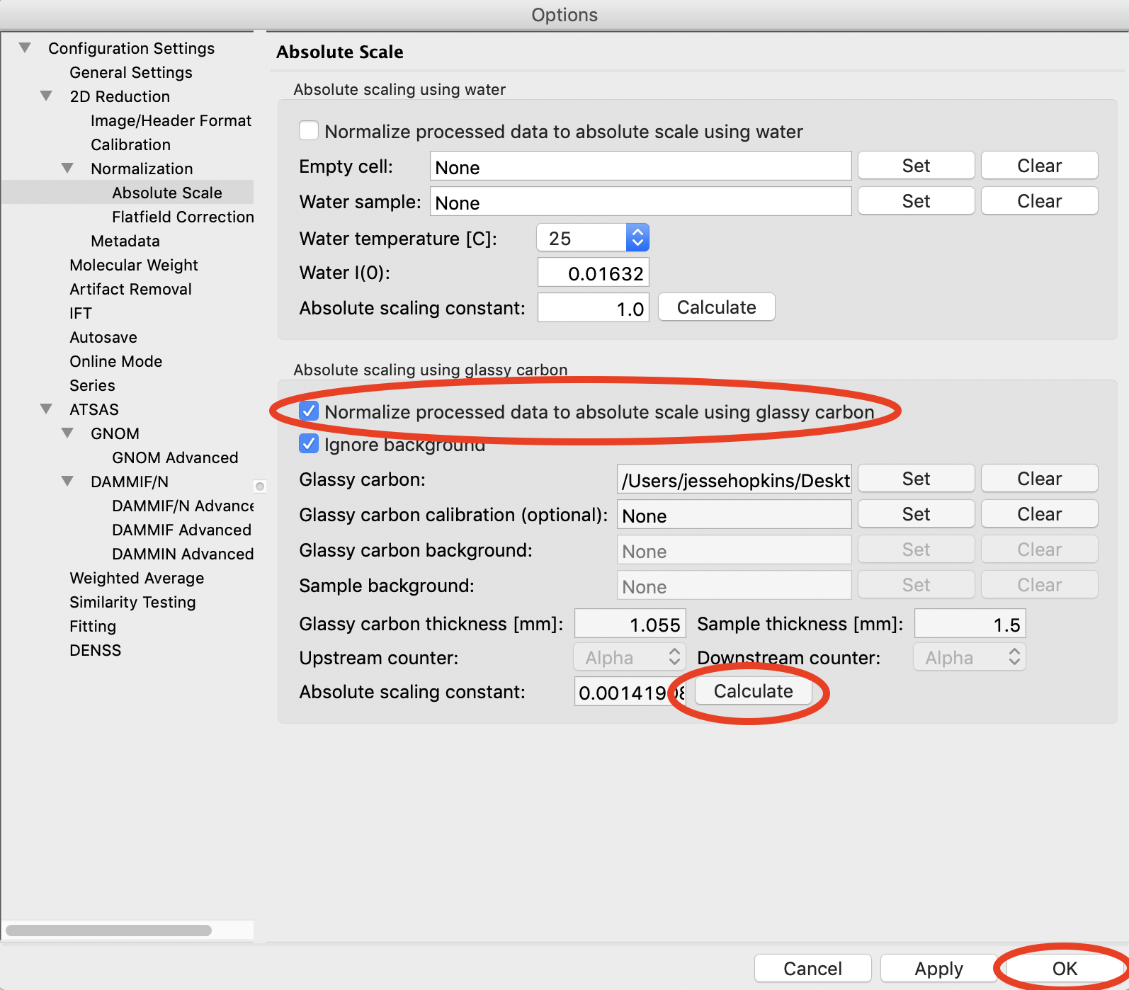
5. Click on the Absolute Scale section in the options list on the left.

   

6. Click on the Glassy carbon “Set” button and select the A_glassy_carbon_41_001_0000.dat file.

7. Set the Sample thickness to 1.5 mm.

   

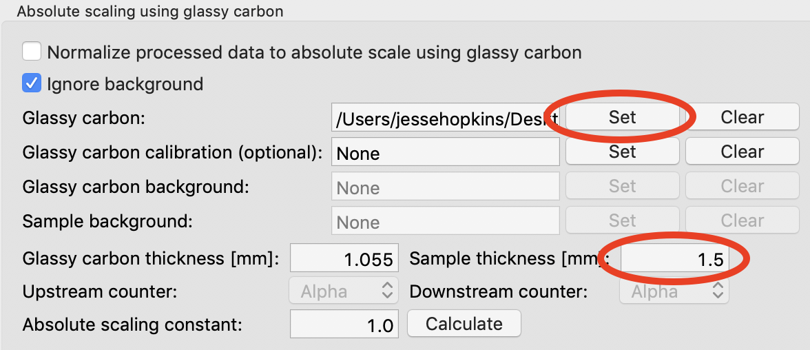
8. Click “Calculate” button. You should get something near 0.0014.

   • Note: It is important that you not change your normalization settings once you have set the absolute scaling constant. If you do, you will have to recalculate the absolute scaling constant. Also, make sure absolute scale is turned off before you calculate the scale constant, otherwise you will get a bad scaling constant (see the manual for details).

9. Check the “Normalize processed data to absolute scale using glassy carbon” checkbox.

10. Click “OK” to exit the advanced options panel, saving the changes.

    

11. Save the settings for future use.

The full, NIST recommended approach:

Important note: All of the normalization (including flux, transmission, etc) happens through the absolute scale panel. You shouldn’t have anything set in the Normalization panel (unless you are doing something like subtracting off a constant pedestal from the image).

1. Load/use the settings from part 4 (without absolute scale set from water, part 5).

2. Open the Options window by selecting “Advanced Options” in the Options menu.

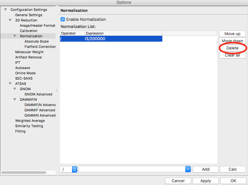
3. Click on the Normalization section in the options list on the left.

4. Remove any/all items in the Normalization List by highlighting them in the list and clicking the “Delete” button.

   

5. Turn off any absolute scaling already in place.

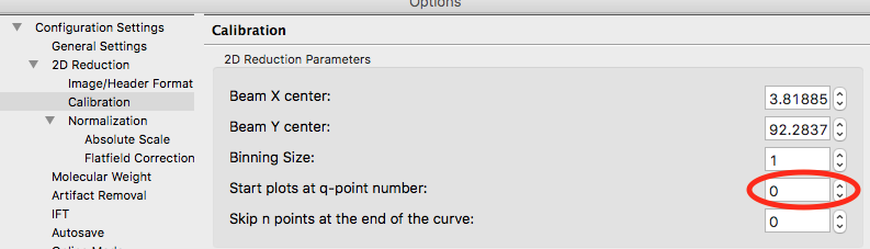
6. Click on the Calibration section in the options list on the left.

7. Change the “Start plots at q-point number” to 0.

   

8. Click “OK” to exit the advanced options window and save the changes.

9. Plot the glassy_carbon_41_001_0000.tiff file.

   • Tip: Section 1 Part 1 of this tutorial document teaches you how to do this.

10. Save the glassy_carbon profile in the calibration_data folder.

11. Plot, average, and save the vac_37_001_000x.tiff and ** MT2_48_001_000x.tiff ** files, where x is 0-9.

    • Tip: Because you aren’t normalizing by beam intensity, these averages may have profiles that are not similar (see Section 1 Part 6). In that case, average just the similar profiles.

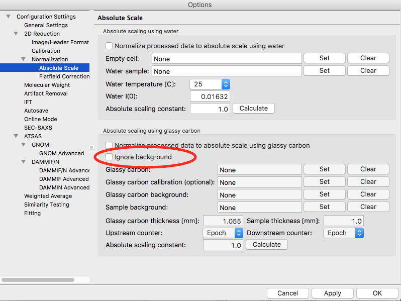
12. Open the Options window and select the Absolute Scale section.

13. Uncheck the Ignore background checkbox.

    

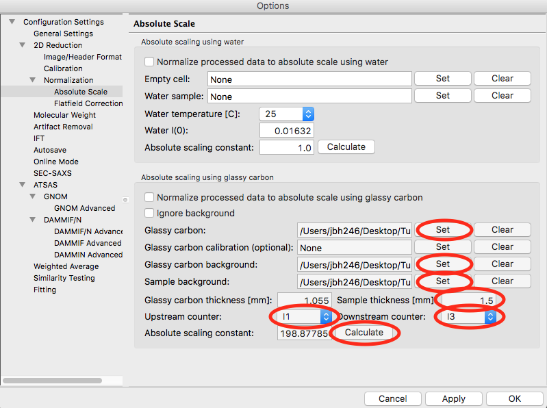
14. Click the Glassy carbon “Set” button and select the glassy_carbon_41_001_0000.dat file.

15. Click the Glassy carbon background “Set” button and select the A_vac_37_001_0000.dat file.

16. Click the Sample background “Set” button and select the A_MT2_48_001_0000.tiff file.

17. Set the Sample thickness to 1.5 mm.

18. Set the Upstream counter to I1.

19. Set the Downstream counter to I3.

20. Click the “Calculate” button. You should get an absolute scaling constant near 198.

    • Note: This approach will only work if the .dat files you select for the glassy carbon, glassy carbon background, and sample background contain the upstream and downstream counter values. This happens automatically with RAW. Otherwise, you should use images, which will have more noise, but should allow RAW to find all of the appropriate counter values.
    • Note: It is important that you not change your normalization settings once you have set the absolute scaling constant. If you do, you will have to recalculate the absolute scaling constant. Also, make sure absolute scale is turned off before you calculate the scale constant, otherwise you will get a bad scaling constant (see the manual for details).

    

21. Check the “Normalize processed data to absolute scale using glassy carbon” checkbox.

22. Click on the Calibration section in the options list on the left.

23. Change the “Start plots at q-point number” to 13.

24. Click “OK” to exit the advanced options panel, saving the changes.

25. Save the settings for future use.

Comparison note:

We find that for the example data given here, the two methods of glassy carbon calibration agree within ~1.5%. The best approach depends on how strong your background scattering is relative to the rest of the scattering in the system.