Pair-distance distribution analysis – GNOM in RAW
The first step in most advanced data processing is to calculate the P(r) function, the Fourier transform of I(q). This cannot be calculated directly from the scattering profile, so indirect Fourier transform (IFT) methods are typically used. The most common such method is implemented in the GNOM program from the ATSAS package. We will use RAW to run GNOM. Note that you need ATSAS installed to do this part of the tutorial.
This tutorial covers how to use RAW for doing an IFT. This is not a tutorial on basic principles and best practices for doing an IFT or analysis of the resulting P(r) function. For that, please see the SAXS tutorial.
A video version of this tutorial is available:
The written version of the tutorial follows.
Open RAW. The install instructions contain information on installing and running RAW. If RAW is already open, clear all loaded data in RAW.
Open the glucose_isomerase.dat file in the Tutorial_Data/reconstruction_data folder.
Right click on the glucose_isomerase profile in the Profiles list and select “IFT (GNOM)”.
- Note: RAW will automatically try to find an appropriate maximum dimension (Dmax) by running the DATGNOM program from the ATSAS software package.
- Troubleshooting: If you do not have the GNOM option in the right click menu, RAW does not know where your ATSAS programs are installed. If you installed the ATSAS programs after starting RAW, restart RAW and it will attempt to automatically find them. If that has failed, go to the Options->Advanced Options menu and choose the ATSAS settings (“ATSAS”). Uncheck the option to “Automatically find the ATSAS bin location”, and specify the location manually.
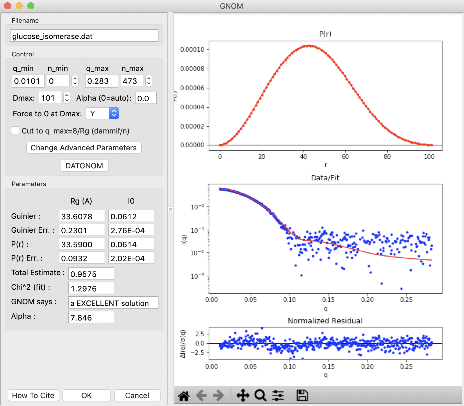
The GNOM panel has plots on the right. These show the P(r) function (top panel), the data (middle panel, blue points) and the fit line (middle panel, red line), and the fit residual (bottom panel).
- Note: The fit line is the Fourier transform of the P(r) function, and is also called the regularized intensity.
On the left of the GNOM panel are the controls and the resulting parameters. You can alter the data range used, the Dmax value, whether the solution is forced to zero at Dmax, and the alpha value used.
- Tip: The Guinier and P(r) Rg and I(0) values should agree well for mostly rigid particles. The total estimate varies from 0 to 1, with 1 being ideal. GNOM also provides an estimate of the quality of the solution. You want it to be at least a “REASONABLE” solution.
Try varying the Dmax value up and down in the range of 80-110. Observe what happens to the P(r) and the quality of the solution.
- Note: Dmax is in units of Å.
Return the Dmax value to that found by DATGNOM by clicking the “DATGNOM” button. Dmax should be 101. By default, GNOM forces the P(r) function to zero at Dmax. For a high quality data set and a good choice of Dmax, P(r) should go to zero naturally. Change the “Force to 0 at Dmax” option to “N”.
- Try: Vary Dmax with this option turned off.
Reset it so that the P(r) function is again being forced to zero at Dmax.
RAW makes it easy to truncate your data to a qmax of 8/Rg, which is the recommended maximum q value for bead model reconstructions with DAMMIF/N. Check the ‘Cut to q_max=8/Rg’ box to truncate the data.
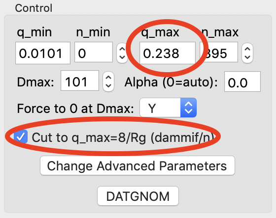
- Note: The qmax goes from 0.283 to 0.238 when you check the box.
- Tip: For electron density reconstruction with DENSS use the full available q range.
Click “OK” to exit the panel and save the IFT to the RAW IFTs panel and plot.
- Tip: After exiting the IFT panel, note that data from the IFT shows up in the Information panel.
Click on the IFTs Control and Plot tabs. This will display the GNOM output you just generated. Save the glucose_isomerase.out item in the reconstruction_data folder.
- Note: This saved file is all of the GNOM output, in the GNOM format. It can be used as input for any program that needs a GNOM .out file.