Indirect Fourier Transform (IFT) and the P(r) function

This tutorial covers basic principles and best practices for doing an Indirect Fourier Transform (IFT) to get a P(r) function. This is not a tutorial on how to use RAW for this type of analysis. For that, please see the RAW tutorial for GNOM and BIFT.

Overview

The SAXS scattering profile is measured in reciprocal distance space, as I(q) where q has units of one over distance (usually 1/Angstrom or 1/nm). We can apply a Fourier transform to the data to get information in real space about the macromolecule, as:

\[P(r) = \frac{r^2}{2\pi^2} \int_0^{\infty} q^2I(q) \frac{\sin(qr)}{qr}dq\]

This produces the P(r) function, also called the pair distance distribution function. Essentially, the P(r) function is the r² weighted histogram of all possible pairs of electrons in the sample.

Why do we do an IFT?

The P(r) function contains valuable information about the shape and size of a macromolecule. First, in doing the P(r) function we get an estimate of the maximum dimension of the macromolecule (D_max). It also provides another, potentially more accurate, way to calculate the R_g and I(0). The shape of the P(r) function can also be directly interpreted in terms of the shape of the macromolecule, providing information about the overall shape, such as globular vs. rod-like, or whether the macromolecule contains multiple domains. Also, the P(r) function and derived parameters such as D_max are required for many advanced analysis techniques including ab-initio reconstructions of the shape.

Additionally, the P(r) function is sensitive to data quality issues, particularly aggregation and interparticle interference. Thus, doing an IFT is another quality check on your data. If you cannot obtain a good P(r) function, then your data probably has one of those issues and usually should not be used for further analysis.

How do we do an IFT?

The equation above cannot be used to directly calculate the P(r) function. The finite extent of our measurement (and measurement noise) means that a direct Fourier transform of I(q) will distort the true P(r) function by introducing truncation artifacts. Instead, the typical approach is to fit the P(r) function against the data. First, you generate the scattering intensity for a given P(r) function as:

\[I(q) = 4\pi \int_0^{D_{max}} P(r) \frac{\sin(qr)}{qr}dr\]

Using this equation you generate the P(r) function that yields the best fit to the data. The fitting criteria include both the actual fit, usually as measured by \(\chi^2\), and regularization parameters. These regularization parameters allow you to add back in information to improve the P(r) function. Typical examples of the regularization parameters include perceptual criteria such as:

• Smoothness of the P(r) function.

• Positivity of the P(r) function.

• Whether the solution changes significantly when changing the weighting of the regularization parameters.

Determining a P(r) function in this way thus requires determining three things:

1. The maximum dimension, D_max, of the sample, as that determines the upper bound of the integral above.

2. The weighting parameter, usually called \(\alpha\), that determines the relative contribution of \(\chi^2\) and the perceptual criteria to the overall fit quality.

3. The P(r) function that yields the best fit to the data, given the particular D_max and \(\alpha\) values.

This is a complicated problem, and there are a number of different programs out there for finding a P(r) function. These programs all typically involve searching a set of possible D_max values and \(\alpha\) values to find which yields the best overall fit. RAW natively supports one method for finding the P(r) function, the Bayesian Indirect Fourier Transform (BIFT) [1], which provides a completely automated determination of D_max and \(\alpha\).

The most popular method for determining the P(r) function is the GNOM [2] software in the ATSAS package, which RAW provides an interface to if ATSAS is installed. Below we discuss how to determine a good P(r) function using GNOM, after discussing the criteria for a good P(r) function.

Criteria for a good P(r) function

We employ the following criteria to determine if a P(r) function is good:

1. The P(r) function falls gradually to zero at \(\mathbf{D_{max}}\).

2. The P(r) function fits the measured scattering profile.

3. The P(r) function goes to zero at \(\mathbf{r=0}\) and \(\mathbf{r=D_{max}}\).

Additionally, the following criteria usually apply:

1. The \(\mathbf{R_{g}}\) and I(0) from the Guinier fit and the P(r) function agree well.

2. The P(r) function is always positive.

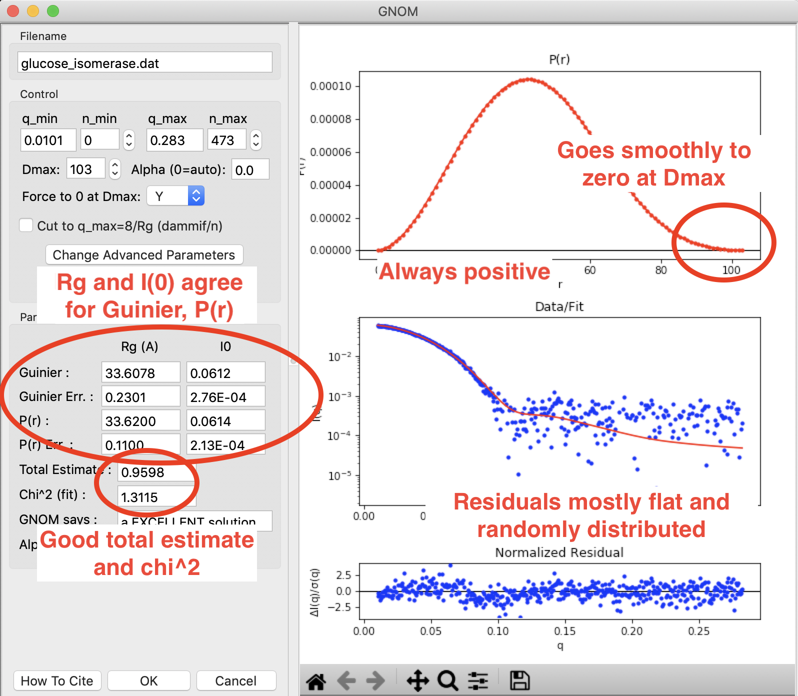
A P(r) function done in RAW using GNOM for glucose isomerase (available in the RAW Tutorial data). This shows what a good P(r) function looks like. The function goes smoothly to zero at D_max, it is always positive, there is good agreement between the Guinier and P(r) R_g and I(0) values, and the residuals are mostly flat and randomly distributed. You can see a small systematic deviation in the residuals below q~0.125. This could be smoothed out by reducing the \(\alpha\) value, which may be slightly over weighting the regularization parameters vs. the actual fit to the data.

A more thorough discussion of each criterion is given below.

The P(r) function falls gradually to zero at D_max

This is perhaps the most important and most subjective criterion for determining whether you have a good P(r) function. The idea is straightforward: macromolecules do not have perfectly sharp boundaries. Because they have side chains that stick out, and have some amount of flexibility in solution (even if limited to solvent exposed side chains), there is no distance at which you go from many electrons pairs to no electron pairs within the macromolecule. As such, the P(r) function should gradually approach zero at the maximum dimension, rather than being cut off.

Essentially, if this criterion is met you have picked an appropriate D_max for the system. If you underestimate the D_max, then the P(r) function has an abrupt descent to zero, while an overestimated D_max usually shows an oscillation about zero. This is shown in the figure below.

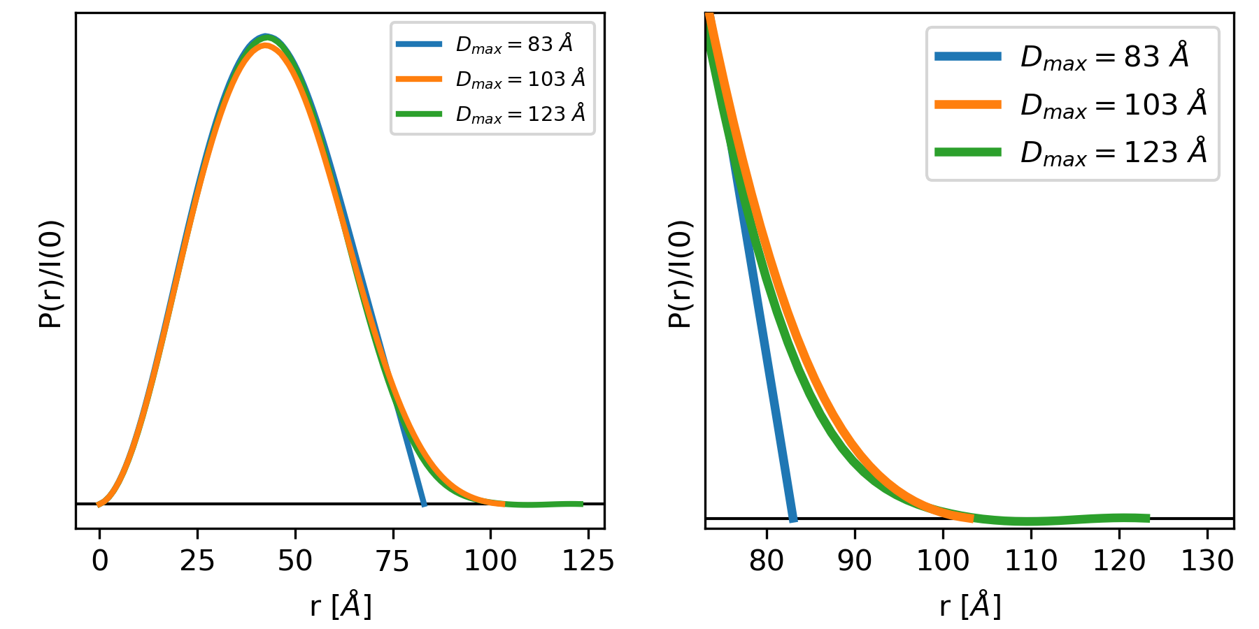
The left and right plots show three different P(r) functions for the same protein (glucose isomerase, available in the RAW Tutorial Data). The difference between the three is the D_max, which is either 83 (blue), 103 (orange) or 123 (green) Angstrom. The left plot shows the full P(r) function. The different D_max values yield similar P(r) functions, so much so that they end up plotted on top of each other for most of their r values. The right plot is the same functions showing just the end, as P(r) approaches zero at D_max.

In the plot above, we can clearly see that for a D_max of 83, the P(r) function is forced abruptly down. For a D_max of 103, the function has a smooth approach to zero. For a D_max of 123 the function reaches zero and then oscillates about it. From this we can conclude that 103 is a good value for D_max, whereas 83 is underestimated and 123 is overestimated.

The P(r) function fits the measured scattering profile

This criterion is straightforward. The transformation of the P(r) function to I(q) should fit the measured scattering profile. This can be evaluated both through the \(\chi^2\) value of the fit, which should be close to 1, and the normalized residuals between the fit and the data, which should be flat and randomly distributed about zero.

The P(r) function goes to zero at \(\mathbf{r=0}\) and \(\mathbf{r=D_{max}}\).

The reason for this criterion is straightforward. The P(r) function should go to zero at r=0 because it is the number of electron pairs in the macromolecule. As r decreases, the number of electron pairs decreases until you reach an r smaller than the size of an electron, at which point there are no pairs left and thus P(r) must go to zero at \(r=0\). The P(r) function should go to zero at \(r=D_{max}\) because D_max is the maximum dimension of the particle. Beyond that distance there should be no electron pairs in the particle. This criterion is usually enforced by conditions in the IFT calculation.

The R_g and I(0) from the Guinier fit and the P(r) function agree well

The R_g and I(0) values can be determined directly from the P(r) function. This provides a complementary approach to the Guinier fit. For well behaved rigid systems, R_g and I(0) should agree well between both methods. If they do not, it may suggest a problem in either the Guinier fit or the P(r) function. However, for flexible and disordered systems, it has been observed that the P(r) R_g and I(0) values are characteristically larger, and more reliable, than the Guinier R_g and I(0) values [3].

The P(r) function is always positive

This criterion usually applies, as for most macromolecules the presence of a negative number of electron pairs has no meaning. However, when dealing with membrane proteins that are encapsulated in lipids or detergents, this criterion is no longer valid. In those cases, the lipid/detergent may have a lower electron density than the buffer. As scattering is measured relative to the solvent, this lower density will appear as negative electron pairs in the P(r) function. For example, proteins embedded in lipid nanodiscs have a characteristic dip in the P(r) function that can go negative.

Determining a good P(r) function using GNOM

While it takes some practice to learn how to properly evaluate the P(r) function, there is a set of steps that I regularly follow when creating a P(r) function using GNOM via the RAW interface:

1. Open the GNOM interface. It defaults to what GNOM thinks is a reasonable D_max (using datgnom).

2. If necessary, set the starting q value for the P(r) function to match that of the Guinier fit (newer versions of RAW do this automatically).

3. Set the D_max value to 2-3 times larger than the initial value.

4. Look for where the P(r) function drops to 0 naturally. Set the D_max value to this point.

5. Turn off the force to zero at D_max condition.

6. Tweak D_max up and down until it naturally goes to zero (with the force to zero turned off).

7. Turn the force to zero at D_max condition back on.

8. If needed, truncate the P(r) function to a maximum q of 8/R_g, or 0.25-0.3 1/Angstrom, whichever is smaller, if using for bead model reconstructions with DAMMIF/N. You may have to tweak the D_max a bit after truncation.

If you have good quality data, this ought to produce a good P(r) function.

Note that even for good quality data with a mostly rigid globular macromolecule like glucose isomerase (shown in the plots above), there usually isn’t a single right value of D_max. For this data, a best case scenario, you could reasonably pick a D_max value from ~99-104, which is a 5% variation. For macromolecules with more flexibility, D_max is even more poorly defined. As a rule of thumb, D_max is usually never determined to better than 5%, sometimes the uncertainty is closer to 10%.

Other tips:

• If the residual has too much systematic deviation, you can manually set the \(\alpha\) to something smaller than the automatic value. Start with half the automatically determined value, and tweak from there.

• Don’t forget to check that the R_g and I(0) values agree (if you have a rigid system). Generally speaking, increasing D_max will increase the P(r) R_g and I(0) values, so that can help guide your choice of D_max.

• Don’t truncate your P(r) function for electron density reconstructions with DENSS.

What is a bad P(r) function, and what does it mean?

Even if you follow all of the guidelines above, sometimes you can end up with a bad P(r) function. Typically what bad means is one of two things:

1. You can’t find a good D_max value. You keep increasing D_max and the P(r) function never smoothly goes to zero.

2. If you increase D_max the P(r) function goes negative.

In these cases, it is most likely that your data has a problem. The figure below gives a quick summary of the most common pathologies, more detail is available in the sections below.

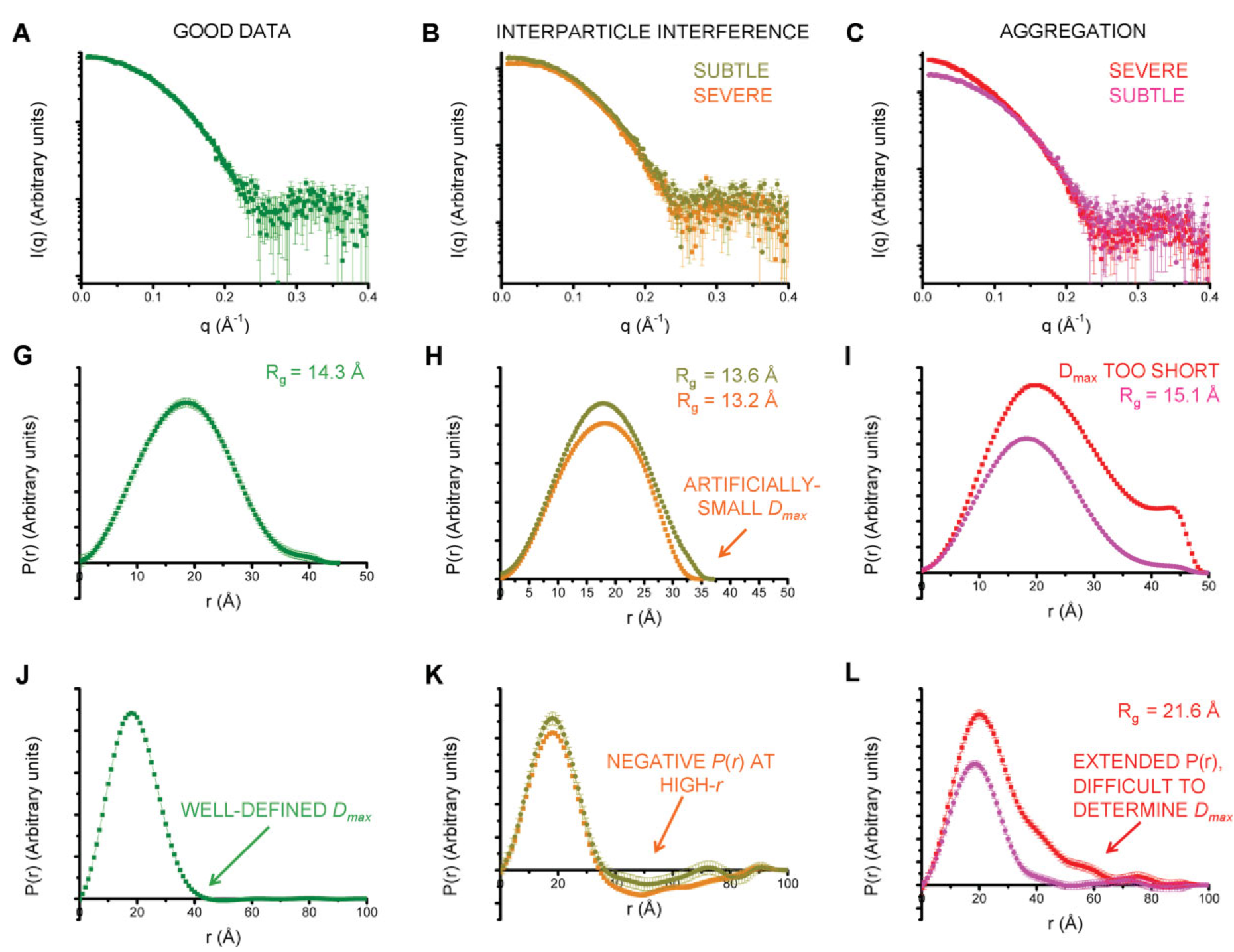
Figure 3 from [4]. A, G, and J show a good (monodisperse) scattering profile and P(r) function. B, H, and K show a scattering profile and P(r) function with varying degrees of interparticle interference. C, I, and L show a scattering profile and P(r) function with varying degrees of aggregation. the middle row shows the effect on the P(r) function, while the last row shows that to really judge the effect of the change on the P(r) function you should extend the D_max value out significantly.

Note that both pathologies are easiest to see when you plot the P(r) function well past the point where you think the correct D_max value is (panels J-L in the above figure). This means that it is important to always extend the D_max value when generating your P(r) function to verify that the P(r) function stays flat and close to zero (usually small oscillations about zero), as in panel J, rather than dipping negative (panel K, repulsive interparticle interference) or staying slightly positive (panel L, aggregation).

Aggregation

Aggregation in solution means some amount of larger particles are present. The presence of these larger particles causes the D_max to be hard to determine. Typically this manifests as there being a significantly extended tail on the P(r) distribution, which does not fall to zero naturally regardless of the chosen D_max. The P(r) function calculated R_g and I(0) will also be larger than they would be for the monodisperse sample.

Small amounts of aggregation can look similar to the P(r) function for a flexible system, so other methods should be used to determine the true state of the system. The Guinier analysis will usually reveal the presence of aggregates, and Kratky plot will show if the system is flexible. If you are unsure whether your P(r) function is showing aggregation or flexibility, check with these other techniques.

Interparticle interference

Interparticle interference usually manifests as repulsion in solution. This repulsive effect manifests as an artificially small D_max. The P(r) function calculated R_g and I(0) values are reduced compared to what they would be for the non-interacting sample.

Since you usually don’t know the D_max of your sample prior to making the measurement, it can be hard to tell if the D_max is artificially small. In this case, the easiest way to see this effect is to extend the D_max out past what you found to be a ‘good’ D_max. If the P(r) function goes and stays negative, as in K of the above figure, then you have a repulsive interaction. If it stays near zero (possibly with some small oscillation about zero), as in J of the above figure, then you are not seeing a repulsive interaction.

How to interpret features of a P(r) function

The P(r) function provides a significant amount of information on particle shape and size in solution. The easiest parameters to interpret are the D_max, R_g, and I(0), which all inform on particle size. The D_max is simply the maximum dimension of the particle. The R_g is the radius of gyration, and I(0) is the scattering at zero angle, which is proportional to the molecular weight and concentration. Beyond these parameters, the shape of the P(r) function contains significant information about the particle shape. This is seen clearly in the plot of P(r) functions for different geometric bodies shown below.

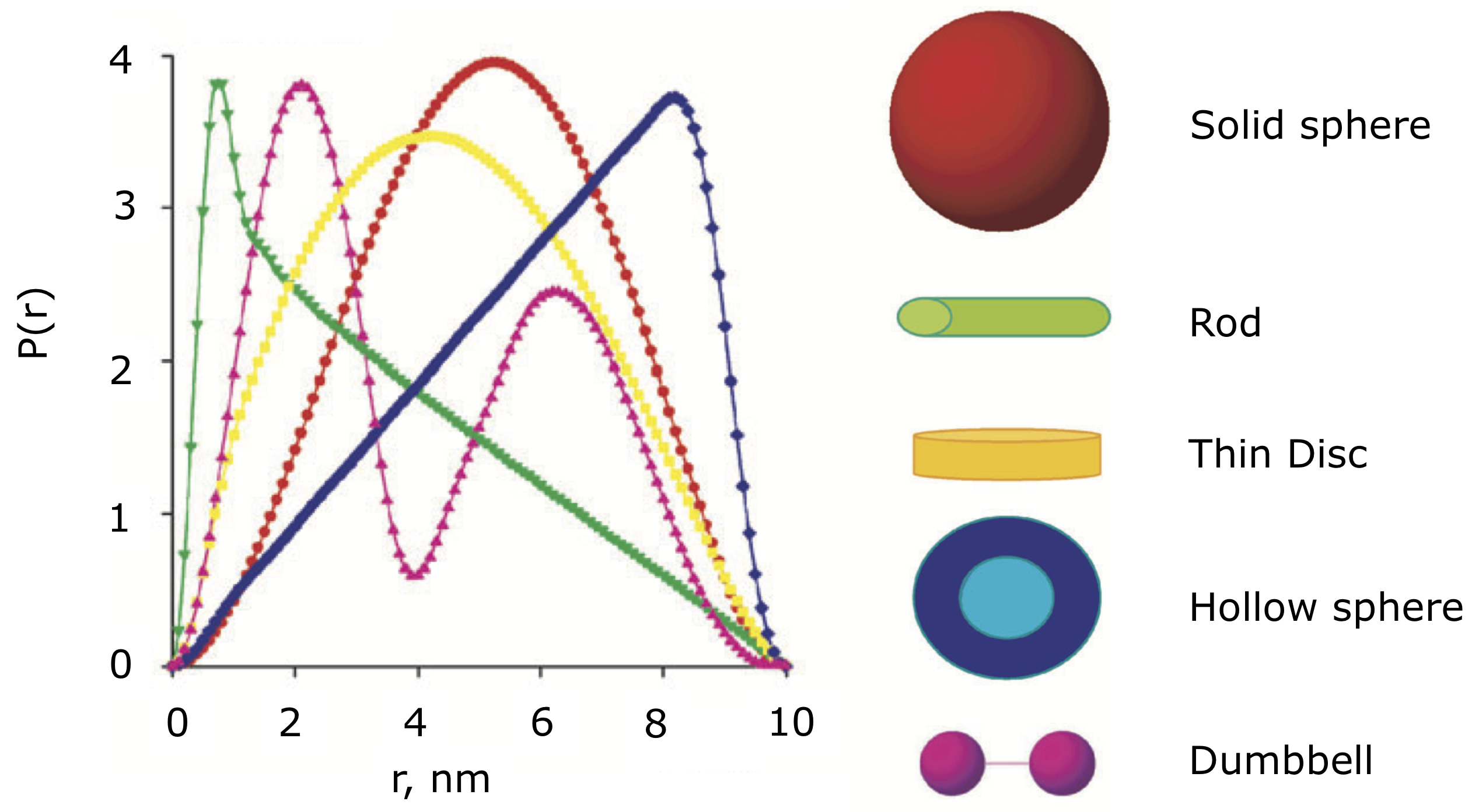
P(r) functions for geometric bodies, adapted from figure 5 of [5].

In the above figure, there are several things worth noting:

1. In the P(r) function for a long rod, the initial peak at short distance comes from electron pairs across the short dimension of the rod. The long extend tail comes from electron pairs along the length of the rod.

2. In the P(r) function for a dumbbell, the peak at lower r comes from the electron pairs within each individual domain of the dumbbell. The peak at longer distance comes from the electron pairs between the two domains of the dumbbell.

3. For the hollow sphere, the peak at long distance is coming from the electron pairs across the diameter of the sphere.

While macromolecules do not have P(r) functions that exactly match those of geometric bodies, the dominant features of the P(r) function can be used to determine overall shape characteristics of the macromolecule. Most usefully:

• Globular proteins tend to have P(r) functions similar to that of a solid sphere.

• Long rigid rod-like systems, like duplex DNA, have P(r) functions very similar to that of a long rod.

• Multi-domain proteins have two peaks, like that of a dumbbell. However, as the domains are not usually symmetric in size or widely separated, the peaks are usually more of a strong peak and an overlapping shoulder peak.

The plot below shows the P(r) function for several actual macromolecules.

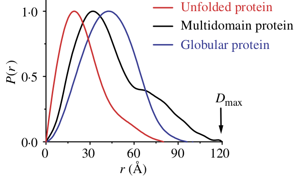
P(r) functions for flexible (unfolded), multidomain, and globular proteins. Figure 24 in [6].

FAQ

Is a small change in D_max significant?

Small changes in D_max are usually not significant. Even for good quality data with a mostly rigid globular macromolecule like glucose isomerase (shown in the plots above), you could reasonably pick a D_max value from ~99-104, which is a 5% variation. For macromolecules with more flexibility, D_max is even more poorly defined. As a rule of thumb, D_max is usually never determined to better than 5%, sometimes the uncertainty is closer to 10%.

My P(r) function goes negative. Is that okay?

Generally speaking, no. However, if you have a system that is detergent or lipid bound, such as a protein embedded in a nanodisc, then you may see a negative dip in your P(r) function.

References

1. Hansen, S. J. Appl. Crystallogr.(2000) 33, 1415-1421. DOI: 10.1107/S0021889800012930

2. Svergun D.I. (1992). J. Appl. Crystallogr. 25, 495-503. DOI: 10.1107/S0021889892001663

3. Kikhney, A. G. & Svergun, D. I. (2015). FEBS Lett. 589, 2570–2577. DOI: 10.1016/j.febslet.2015.08.027

4. Jacques, D. A. & Trewhella, J. (2010). Protein Sci. 19, 642–657. DOI: 10.1002/pro.35

5. Svergun, D. I. & Koch, M. H. J. (2003). Reports Prog. Phys. 66, 1735–1782. DOI: 10.1088/0034-4885/66/10/R05

6. Putnam, C. D., Hammel, M., Hura, G. L. & Tainer, J. a (2007). Q. Rev. Biophys. 40, 191–285. DOI: 10.1017/S0033583507004635