Loading configuration files and images, creating subtracted scattering profiles, saving profiles

1. Open RAW. The install instructions contain information on installing and running RAW.

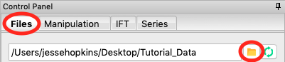
2. In the files tab, click on the folder button and navigate to the Tutorial_Data/standards_data folder. Click the open button to show that folder in the RAW file browser.

   

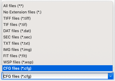
3. At the bottom of the File tab in the Control Panel, use the dropdown menu to set the file type filter to “CFG files (*.cfg)”.

   

4. Double click on the SAXS.cfg file to load the SAXS configuration. This loads the beamline configuration into the program.

   • Note: Any time you are going to process images, you need to load the appropriate configuration!

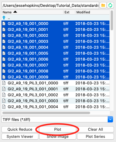
5. Change the file type filter to “TIFF files (*.tiff)”.

6. At the CHESS G1 station, typically ~10 images are collected from a given sample. To load in the 10 images for the glucose isomerase (GI) sample, start by selecting the files GI2_A9_19_001_xxxx.tiff, where xxxx will range from 0000 to 0009. These files are measured scattering from 0.47 mg/ml GI.

   • Tip: you can hold down the ctrl key (apple key on macs) while clicking to select multiple files individually. You can also click on a file, and then shift click on another file to select those files and everything between them.
   • Warning: Don’t load the files with PIL3 in their name. Those are the wide-angle scattering (WAXS) data, which we will process separately later.

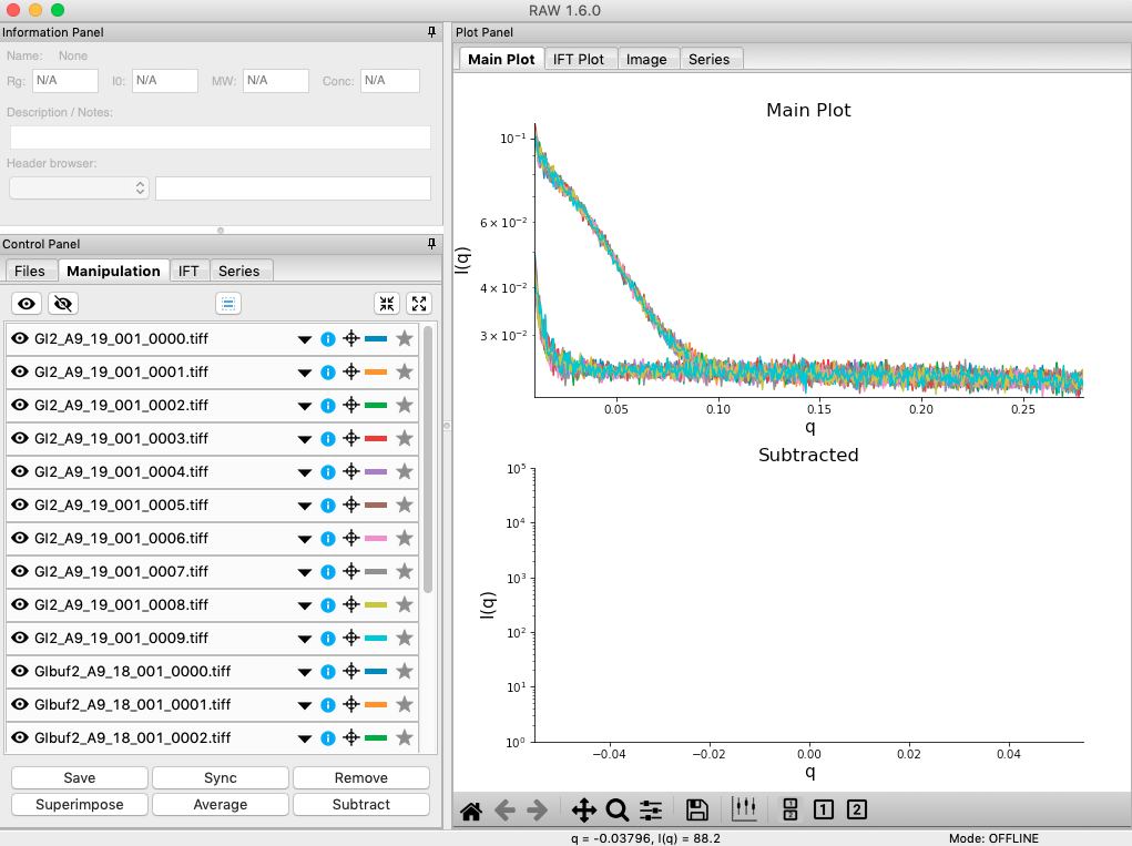
7. Click the plot button to integrate all of the images and plot the integrated scattering profiles on the Main Plot.

   • Note: Typically, once the images are integrated we work only with the scattering profiles. However, it is useful to keep the images around in case you want to reprocess the data.

   

8. Plot the GIbuf2 scattering profiles from the images. These are measured scattering from the matching buffer, without any protein, for the GI sample.

9. Click on the Manipulation tab. This is where you can see what scattering profiles are loaded into RAW, and manipulate/analyze them.

   • Checkpoint: If you’ve successfully loaded the images given, you should see twenty scattering profiles in the manipulation list, with names like GI2_A9_19_001_0000.tiff or GIbuf2_A9_18_001_0000.tif.

   

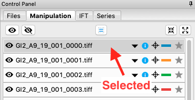
10. Click on a filename to select the scattering profile. The background should turn gray, indicating it is selected.

    

11. Select all of the GI scattering profiles

    • Tip: Again, the ctrl(/apple) key or the shift key can be used to select multiple scattering profiles.
    • Warning: Select only the GI profiles, not the GI buffer profiles.

    

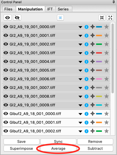
12. Use the average button to average all of the scattering profiles collected into a single curve.

    • Checkpoint: The averaged scattering profile should appear at the bottom of the manipulation list. You may have to scroll down to see it. The filename will be in green, and will start with A_, indicating it is an average scattering profile.

13. Average all of the GI buffer scattering profiles.

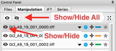
14. In order to see the averaged scattering profiles, you will need to hide the individual profiles from the plot. Clicking on the check box to the left of the filename will show/hide a scattering profile. When the box is checked, the profile is shown on the plot, when it is unchecked, the profile is hidden. Hide all of the profiles except the two averaged curves.

    • Tip: The eye and eye with the x through it at the top of the manipulation panel can be used to show/hide sets of loaded profiles at once. If no profiles are selected, these buttons show/hide all loaded profiles. If some profiles are selected, these buttons show/hide just the selected profiles. Try selecting all but the averaged files and using the show/hide all buttons.

    

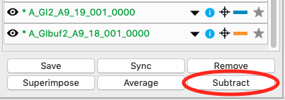
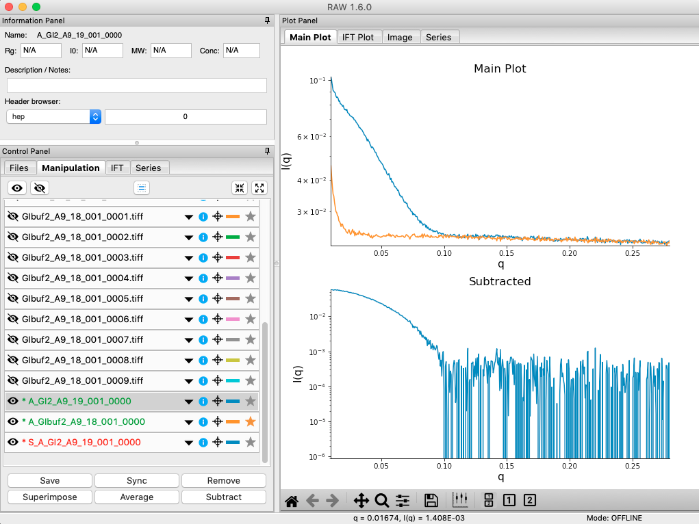
15. Next you need to subtract the buffer scattering profile from the measured protein scattering (which is really the scattering of the protein plus the scattering of the buffer). Star the averaged buffer file, and select the averaged protein file, then click the subtract button.

    

    • Checkpoint: The subtracted scattering profile should be shown in the lower plot. A new manipulation item should be shown in the manipulation menu, with the name in red and a S_ prefix indicating it is a subtracted file.

    

16. You don’t need the individual image scattering profiles any more. Select all of those (but not your averaged or subtracted profiles!) and click remove.

    • Note: This only removes the scattering profiles from RAW. The images on your hard drive are unaffected.

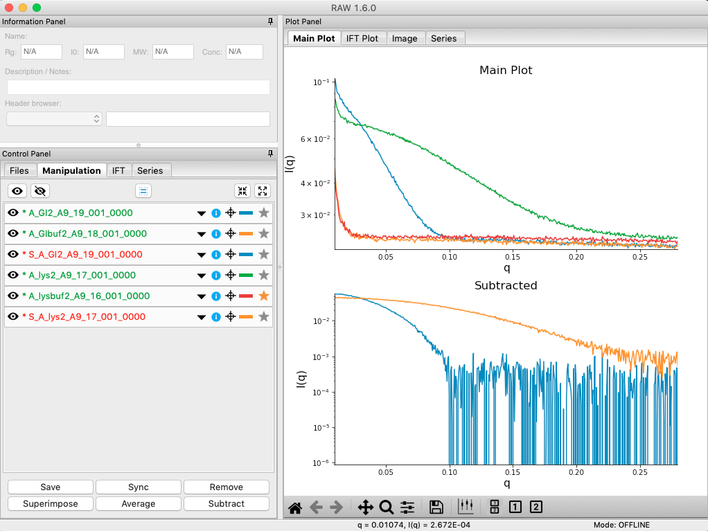
17. Load in the lys2 and lysbuf2 files, average, and subtract to create a subtracted lysozyme scattering profile. The concentration of this sample was 4.27 mg/ml. Remove all of the profiles that are not averaged or subtracted profiles.

    • Tip: In order to tell which curve is which in a plot, click on the target icon in the manipulation list. This should bold that curve in the plot. Click the target icon again to return the curve to normal.

    

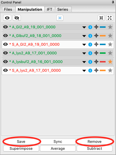
18. We’re done with the averaged profiles. Select all of the averaged profiles and click the “Save” button to save them in the standards_data folder. Note that in the filename in the manipulation list, the * at the front goes away. This indicates there are no unsaved changes to those scattering profiles. You can now remove them.

    • Note: This saves them with a .dat extension. This is the standard format for SAXS scattering profiles, and is also human readable.

    

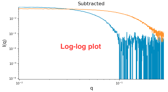
19. Right click on the subtracted plot, move the cursor over ‘Axes’ and select the Log-Log option. Well-behaved globular proteins will intersect the intensity axis roughly perpendicularly.

    • Note: It is best practice to display SAXS data, particularly in publications, on either a semi-log (Log-Lin, default option in RAW) or double-log plot (depending on the features of interest).