Advanced SEC-SAXS processing – Singular value decomposition (SVD) and evolving factor analysis (EFA)
Sometimes SEC fails to fully separate out different species, and you end up with overlapping peaks in your SEC-SAXS curve. It is possible to apply more advanced mathematical techniques to determine if there are multiple species of macromolecule in a SEC-SAXS peak, and to attempt to extract out scattering profiles for each component in an overlapping peak. Singular value decomposition (SVD) can be used to help determine how many distinct scatterers are in a SEC-SAXS peak. Evolving factor analysis (EFA) is an extension of SVD that can extract individual components from overlapping SEC-SAXS peaks.
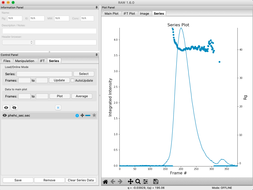
Clear all of the data in RAW. Load the phehc_sec.sec file in the sec_data folder.
- Note: The data were provided by the Ando group at Cornell University and is some of the data used in the paper: Domain Movements upon Activation of Phenylalanine Hydroxylase Characterized by Crystallography and Chromatography-Coupled Small-Angle X-ray Scattering. Steve P. Meisburger, Alexander B. Taylor, Crystal A. Khan, Shengnan Zhang, Paul F. Fitzpatrick, and Nozomi Ando. Journal of the American Chemical Society 2016 138 (20), 6506-6516. DOI: 10.1021/jacs.6b01563
Right click on the phehc_sec.sec item in the Series list. Select the “SVD” option.
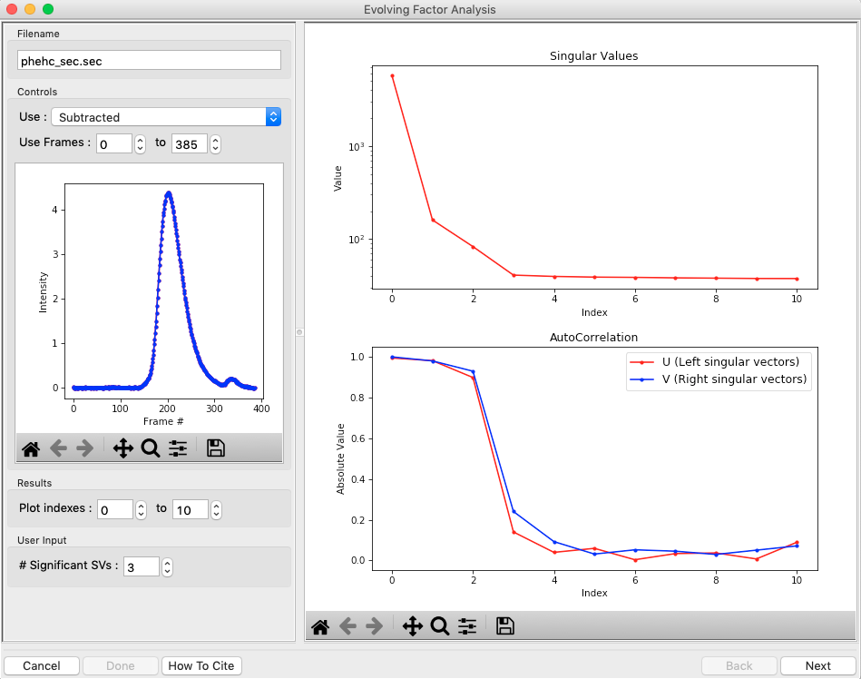
The SVD window will be displayed. On the left are controls, on the right are plots of the value of the singular values and the first autocorrelation of the left and right singular vectors.
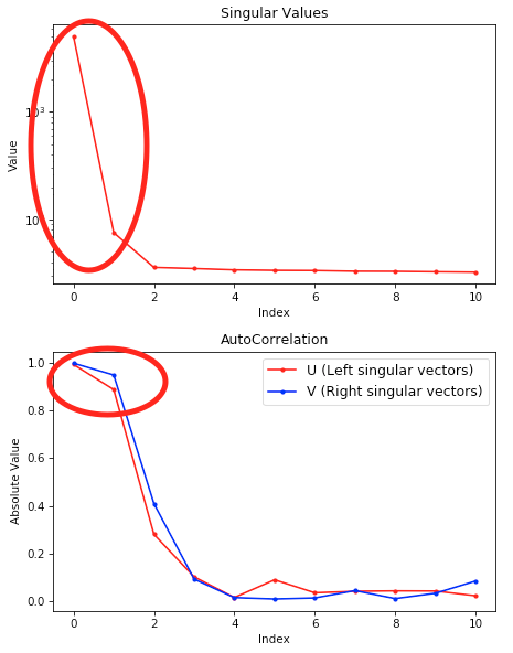
- Note: Large singular values indicate significant components. What matters is the relative magnitude, that is, whether the value is large relative to the mostly flat/unchanging value of high index singular values.
- Note: A large autocorrelation indicates that the singular vector is varying smoothly, while a low autocorrelation indicates the vector is very noisy. Vectors corresponding to significant components will tend to have autocorrelations near 1 (roughly, >0.6-0.7) and vectors corresponding to insignificant components will tend to have autocorrelations near 0.
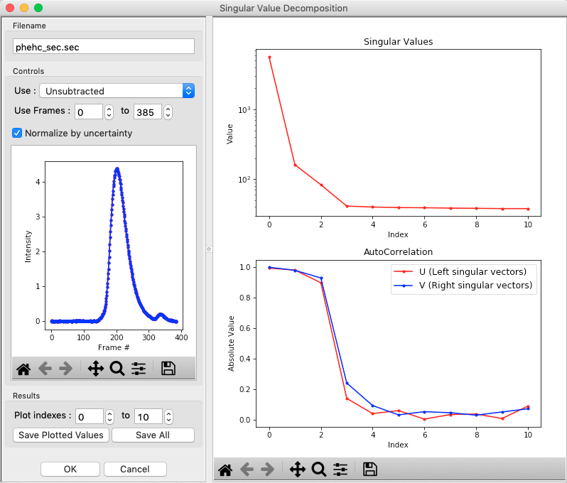
Adjust the starting frame number to 100, the ending frame number to near 300, and switch to using Subtracted data.
- Note: The blue points are in the plot on the left are the region being used for SVD, while the red points shows the rest of the SEC-SAXS curve.
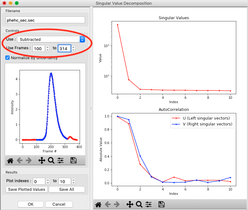
We have now isolated the peak. Looking at the top plot, we see there are two singular values significantly above the baseline level, and from the autocorrelation we see two values with both left and right singular vectors autocorrelations near 1. This indicates that there are two scattering components in the peak, even though there are no obvious shoulders in the region we selected
- Try: Adjust the starting and ending values and seeing how that changes the SVD results. Is there a region of the peak you can isolate that has just one significant component?
- Note: Normally, changing between Unsubtracted and Subtracted SEC-SAXS profiles should remove one significant singular value component, corresponding to the buffer scattering. In this data, you will see no difference, as the profiles used to produce the SEC-SAXS curve were already background subtracted.
- Note: You can save the SVD plots by clicking the Save button, as with the plots in the main RAW window. You can save the SVD results, either just the plotted values or all of the values, using the two Save buttons in the SVD panel.
Close the SVD window by clicking the OK button.
We will now use EFA to attempt to extract out the two scattering components in the main peak in this data. Right click on the phehc_sec.sec item in the Series list. Select the “EFA” option.
For successful EFA, you want to use Subtracted data, and you typically want to have a long buffer region before and after the sample. For this data set, using the entire frame range (from 0 to 385) is appropriate. With other data sets, you may need to change the frame range to, for example, remove other, well separated, peaks from the analysis.
RAW attempts to automatically determine how many significant singular values (SVs) there are in the selected range. At the bottom of the control panel, you should see that RAW thinks there are three significant SVs in our data. For this data set, that is accurate.
- Note: You should convince yourself of this by looking at the SVD results in the plots on this page, using the same approach as in Steps 3-5 above.
- Note: There is a hint of a fourth component. You can rerun this exercise using four components and see if that changes the results.
Click the “Next” button in the lower right-hand corner of the window to advance to the second stage of the EFA analysis.
- Note: It may take some time to compute the necessary values for this next step, so be patient.
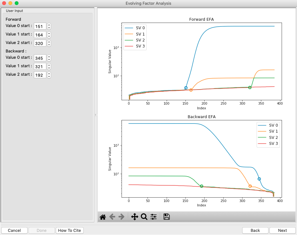
This step shows you the “Forward EFA” and “Backward EFA” plots. These plots represent the value of the singular values as a function of frame.
- Note: There is one more singular value displayed on each plot than available in the controls. This is so that in the following Steps you can determine where each component deviates from the baseline.
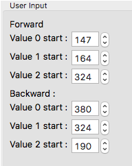
In the User Input panel, tweak the “Forward” value start frames so that the frame number, as indicated by the open circle on the plot, aligns with where the singular value first starts to increase quickly. This should be around 147, 164, and 324.
- Note: For the Forward EFA plot, SVD is run on just the first two frames, then the first three, and so on, until all frames in the range are included. As more frames are added, the singular values change, as shown on the plot. When a singular values starts increasingly sharply, it indicates that there is a new scattering component in the scattering profile measured at that point. So, for the first ~150 frames, there are no new scattering components (i.e. just buffer scattering). At frame ~151, we see the first singular value (the singular value with index 0, labeled SV 0 on the plot) start to strongly increase, showing that we have gained a scattering component. We see SV 1 start to increase at ~167, indicating another scattering component starting to be present in the scattering profile.
In the User Input panel, tweak the “Backward” value start frames so that the frame number, as indicated by the open circle on the plot, aligns with where the singular value first starts to increase quickly, reading the plot left to right (i.e. where it drops back to near the baseline). This should be around 380, 324, and 190.
- Note: For the Backward EFA plot, SVD is run on just the last two frames, then the last three, and so on, until all frames in the range are included. As more frames are added, the singular values change, as shown on the plot. When a singular values starts increasingly sharply (as seen from right to left), it indicates that there is a new scattering component in the scattering profile measured at that point.
- Note: The algorithm for determining the start and end points is not particularly advanced. For some datasets you may need to do significantly more adjustment of these values
Click the “Next” button in the bottom right corner to move to the last stage of the EFA analysis.
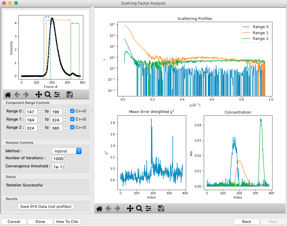
This window shows controls on the left and results on the right. In the controls area, at the top is a plot showing the SEC-SAXS curve, along with the ranges occupied by each scattering component, as determined from the input on the Forward and Backward EFA curves in stage 2 of the analysis. The colors of the ranges correspond to the colors labeled in the Scattering Profiles plot on the top right and the Concentration plot in the lower right. This panel takes the SVD vectors and rotates them back into scattering vectors corresponding to real components.
- Note: This rotation is not guaranteed to be successful, or to give you valid scattering vectors. Any data obtained via this method should be supported in other ways, either using other methods of deconvolving the peak, other biophysical or biochemical data, or both!
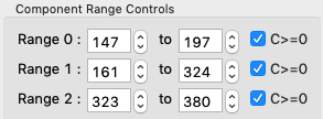
Fine tune the ranges using the controls in the “Component Range Controls” box. Adjust the start of Range 2 down until it overlaps with Range 1.
- Question: What is the effect on the chi-squared plot?
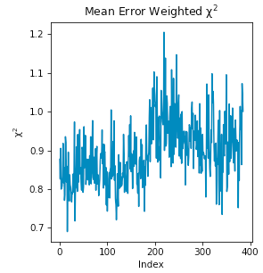
Adjust the starts and ends of Range 0 and the start of Range 1 by a few points until the spikes in the chi-squared plot go away. After these adjustments, Range 0 should be about 147 to 197, Range 1 from 161 to 324, and Range 2 from 323 to 380.
To see these changes on the Forward and Backward EFA plots, click the “Back” button at the bottom right of the page. Verify that all of your start and end values are close to where the components become significant, as discussed in Steps 12 and 13.
Click the “Next” button to return to the final stage of the EFA analysis.
In the Controls box, you can set the method, the number of iterations, and the convergence threshold. As you can see in the Status window, the rotation was successful for this data. If it was not, you could try changing methods or adjusting the number of iterations or threshold.
Examine the chi-squared plot. It should be uniformly close to 1 for good EFA. For this data, it is.
Examine the concentration plot. You’ll see three peaks, corresponding to the concentrations for the three components. In the Range Controls, uncheck the Range 0 C>=0 box. That removes the constraint that the concentration must be positive. If this results in a significant change in the peak, your EFA analysis is likely poor, and you should not trust your results.
- Note: The height of the concentration peaks is arbitrary, all peaks are normalized to have an area of 1.
Uncheck all of the C>=0 controls.
- Question: Do you observe any significant changes in the scattering profiles, chi-squared, or concentration when you do this? How about if you uncheck one and leave the others checked?
Recheck all of the C>=0 controls. You have now verified, as much as you can, that the EFA analysis is giving you reasonable results.
Reminder: Here are the verification steps we have carried out, and you should carry out every time you do EFA:
- Confirm that your selected ranges correspond to the start points of the Forward and Backward EFA values (Steps 12-13).
- Confirm that your chi-squared plot is close to 1, without any major spikes (Step 21).
- Confirm that your concentrations are not significantly altered by constraining the concentration to be positive (Steps 22-23).
Click the “Save EFA Data (not profiles)” to save the EFA data, including the SVD, the Forward and Backward EFA data, the chi-squared, and the concentration, along with information about the selected ranges and the rotation method used.
Click the “Done” button to send the scattering profiles to the Main Plot.
In the main RAW window, go to the Manipulation control tab and the Main plot. If it is not already, put the Main plot on a semi-Log or Log-Log scale.
The three scattering profiles from EFA are in the manipulation list. The labels _0, _1, and _2 correspond to the 0, 1, and 2 components/ranges.
- Note: Regardless of whether you use subtracted or unsubtracted data, these scattering profiles will be buffer subtracted, as the buffer represents a scattering component itself, and so (in theory) even if it is present will be separated out by successful EFA.