Analysis windows
WARNING: The manual is current several versions out of date. While it may still be useful for some users, please refer to the tutorial for the most up-to-date information.
There are a variety of analysis windows in RAW: the Guinier Fit window, the Molecular Weight window, the BIFT window, the GNOM window, the AMBIMETER window, the DAMMIF window, the SVD window, and the EFA window. In this chapter we will cover how to open these windows and carry out the analysis.
Guinier Fit window
Data that has been properly background subtracted can be analyzed in the standard fashion via a Guinier Fit to yield the radius of gyration and the scattering intensity at zero angle. The Guinier Fit window allows you to interactively do the fit.
Opening the Guinier fit window
The Guinier fit window can be opened by selecting a data item in the Manipulation Panel and either right clicking and selecting “Guinier fit” or selecting “Guinier fit” from the “Tools” menu. Whichever data item is selected will be the one that is being analyzed. If multiple items are selected, the first (top item in the list) will be sent to the Guinier Fit panel.
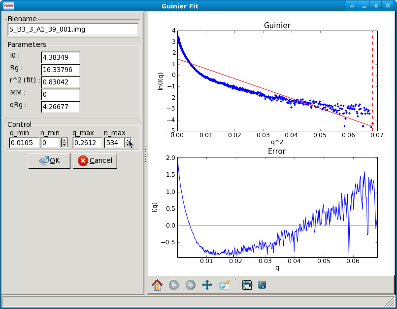
Once the window opens you will see two panels. The left panel has the filename of the data loaded into the Guinier Fit panel, the fit parameters, and the fit controls. The right panel has two plots that show the fit and residual. If no previous Guinier fit analysis has been saved for the data item, the fit range defaults to the whole scattering profile. If a previous Guinier fit analysis was saved for the data item, the fit range will be the range of that analysis.
Once you have completed a satisfactory Guinier fit, clicking the “OK” button will save the fit for the data item selected. That will allow you to save the Guinier analysis parameters when saving all results, view the results in the information window, and save it with the scattering profile if that is saved as a “.dat” file. Clicking the “Cancel” button (or the close window button from the operating system, typically in the upper left or right corner) will exit the window without saving the analysis results.
Note 1: Only one Guinier Fit window can be open at once. If a window is already open and you try to open a new one, it will close the current window and open a new one.
Note 2: RAW will automatically attempt to automatically determine the Rg when the Guinier window is opened, if no previous Guinier fit has been done. If a previous Guinier fit has been done, RAW will set the q min and q max to the previous values.
Guinier Fit Controls
The Guinier Fit Controls allow you to manually set the q_min and q_max values over which the Guinier fit is done. You can do this in two ways. First, if you type a value into the q_min or q_max box and hit enter, RAW will find the nearest q point, and set the q value to that nearest point. Second, you can adjust the n_min and n_max values either by typing an integer value in the appropriate box or using the spin controls. The n_min and n_max controls change the minimum and maximum points of the q vector used (zero indexed), and the q_min and q_max are updated to match. For example if n_min is set to 5 and n_max is set to 130, the 5th indexed point through the 130th indexed point in the q vector (so points 6-131, because of the zero indexing) will be used in the Guinier fit.
The AutoRG button calls a function that attempts to automatically determine the best range of data to use for the Guinier fit. It considers the following criteria: q_min*Rg as small as possible, q_max*Rg as close to 1.3 as possible, smallest fit error in the Rg, smallest fit error in the I(0) possible, r^2 of the fit as close to one as possible, and the largest range of q values used as possible.
Guinier Fit Plots
There are two plots in the Guinier fit window. The top plot is the standard Guinier plot, ln(I(q)) vs. q2, shown in the range of n_min -20 to n_max +3 (if possible) as set in the Guinier Control panel. The scattering profile is marked by the blue points, the fit is shown as the solid straight red line, the fit extrapolated to q=0 is shown by the green dashed line, and the range of the fit, q_min and q_max, are shown by vertical red dashed lines.
The bottom plot has the residual between each point in the scattering profile and the fit, plotted as \(\Delta ln(I(q))\) vs. q2. The red line is a line at zero. Note that the x range of this plot may be slightly reduced compared to the top plot, as it only displays the fit, while the top plot can display points beyond the limits of the fit.
Note: There are no controls available on right click for these plots, but there is a standard plot control bar.
Guinier Fit Parameters
The fit parameters available in the Guinier Fit window are:
- I(0), the extrapolated scattering intensity at zero angle
- Rg, the radius of gyration
- r2 (fit), the r2 value of the fit
- qRg, which is q_min*Rg and q_max*Rg for the left and right boxes respectively.
Molecular weight
Data that has been background subtracted and had a Guinier fit carried out can be analyzed to find the molecular weight of the macromolecule. RAW provides four different ways of calculating the molecular weight, which are described below.
Opening the Molecular Weight Window
The Molecular Weight window can be opened by selecting a data item in the Manipulation Panel and either right clicking and selecting “Molecular Weight” or selecting “Molecular Weight” from the “Tools” menu. Whichever data item is selected will be the one that is being analyzed. If multiple items are selected, the first (top item in the list) will be the one analyzed.
The window has two parts. The top part is a description of the MW methods and a panel with the Guinier fit parameters. The bottom part is four panels providing the calculated MW from each method, and the ability to see more details and learn more about each method. All of the MW methods require a Guinier fit to have been done, as they rely on the I(0) value. Two of the methods require knowing the sample concentration, and the same two methods also depend on (different) calibration of the scattering profile.
Once you are satisfied with the molecular weight analysis, clicking the “OK” button will save the analysis for the data item selected. That will allow you to save the molecular weight analysis parameters when saving all results, view the results in the information window, and save the results with the scattering profile if that is saved as a “.dat” file. Clicking the “Cancel” button (or the close window button from the operating system, typically in the upper left or right corner) will exit the window without saving the analysis results.
Note: Only one molecular weight window can be open at once. If a window is already open and you try to open a new one, it will close the current window and open a new one.
The molecular weight controls
There are several controls available in the molecular weight panel. In the top panel, the Guinier Fit button can be used to open the Guinier panel and (re)analyze the scattering profile using that method, so that an I(0) value is available for the molecular weight panel.
Each of the four lower panels has a “Show Details” and “More Info” button. The “More Info” button simply provides an extended description of the method used, and, when relevant, a citation. The “Show Details” button provides extended information on the parameters used to calculate the MW for a given method. None of these parameters are editable in the molecular weight panel. When the “Show Details” button is clicked, it becomes a “Hide Details” button, which hides the extra parameters.
The concentration box in both the first and fourth panels can have the sample concentration entered, if it has not already been (for example, in the Information panel). These are linked, so that any change to one also changes the other. Sample concentration should be in mg/ml.
The volume of correlation method uses different parameters for Proteins and RNA, and the drop down menu can be used to toggle between those two sets of parameters. The default setting can be changed in the Options window.
If RAW is set to normalize scattering profiles to an absolute scale, the “Intensity on Absolute Scale” box will be checked in the fourth panel. If RAW is not normalizing to an absolute scale, it will be unchecked. If that is set incorrectly for a particular scattering profile for some reason, it can be manually toggled to the correct position.
At the bottom of the window there are three buttons. The “OK” and “Cancel” buttons have been described above. The “Change Advanced Parameters” button opens the Options window, with the Molecular Weight section shown. This allows you to change the parameters used to calculate the molecular weight for each method of calculation.
The molecular weight parameters
There are a number of parameters listed in the molecular weight panel. In the top panel there are:
Filename
Gives the filename of the data item being analyzed.
Guinier parameters
Gives the I(0) and Rg from the Guinier fit.
In the I(0) Ref. MW panel there are:
Concentration
The sample concentration in mg/ml, this field accepts input.
MW
The sample MW calculated by this method, in kDa.
Ref. I(0)
The I(0) of the molecular weight standard set for RAW. This field corresponds to the I(0) field in the “Molecular Weight Estimation Using a Standard” box in the Molecular Weight section of the Options window, and can be changed there or by setting the MW standard.
Ref. MW
The molecular weight of the molecular weight standard set for RAW. This field corresponds to the MW field in the “Molecular Weight Estimation Using a Standard” box in the Molecular Weight section of the Options window, and can be changed there or by setting the MW standard.
Ref. Concentration
The concentration of the molecular weight standard set for RAW. This field corresponds to the Conc. field in the “Molecular Weight Estimation Using a Standard” box in the Molecular Weight section of the Options window, and can be changed there or by setting the MW standard.
File – The data item name of the molecular weight standard set for RAW. This field corresponds to the Filename field in the “Molecular Weight Estimation Using a Standard” box in the Molecular Weight section of the Options window, and can be changed there or by setting the MW standard.
In the Vc MW panel there are:
MW
The sample molecular weight calculated by this method, in kDa.
Vc
The volume of correlation calculated by this method, in Å2.
Qr
The Qr parameter calculated by this method, in Å3.
a
The macromolecular type (protein/RNA) dependent “a” parameter used for the calculation. This field corresponds to the “Protein (RNA) Coef. A” field in the “Molecular Weight Estimation From Volume of Correlation” box in the Molecular Weight section of the Options window, and can be changed there. The value depends on whether Protein or RNA is selected in the drop down menu at the top of this panel.
b
The macromolecular type (protein/RNA) dependent “b” parameter used for the calculation. This field corresponds to the “Protein (RNA) Coef. B” field in the “Molecular Weight Estimation From Volume of Correlation” box in the Molecular Weight section of the Options window, and can be changed there. The value depends on whether Protein or RNA is selected in the drop down menu at the top of this panel.
This panel also has a plot which shows \(\int q I(q) dq\) vs. q, over the q-range of the scattering profile. For this method to be accurate, the integral value needs to have converged at high q (the graph needs to be flat at high q).
In the Vp MW panel there are:
MW
The sample molecular weight calculated by this method, in kDa.
Vp
The Porod volume calculated by direct integration of the scattering profile, in Å3.
Corrected Vp
The corrected Porod volume based on the method described below, in Å3.
Macromolecule Density
The density of the macromolecule, used to calculate the molecular weight. This field corresponds to the “Density” field in the “Molecular Weight Estimation from Corrected Porod Volume” box in the Molecular Weight section of the Options window, and can be changed there.
In the Abs. MW panel there are:
Concentration
The sample concentration in mg/ml, this field accepts input.
MW
The sample MW calculated by this method, in kDa.
# electrons per mass dry macromolecule
The dry mass number density of electrons for the macromolecule, in e-/g. This field corresponds to the “Electrons per dry mass of macromolecule” field in the “Molecular Weight Estimation from Absolute Intensity Calibration” box in the Molecular Weight section of the Options window, and can be changed there.
# electrons per volume of buffer
The number density of electrons for the protein buffer/solvent, in e-/cm3. This field corresponds to the “Electrons per volume of aqueous solvent” field in the “Molecular Weight Estimation from Absolute Intensity Calibration” box in the Molecular Weight section of the Options window, and can be changed there.
Protein partial specific volume
The partial specific volume of the macromolecule, in cm3/g. This field corresponds to the “Partial specific volume of the macromolecule” field in the “Molecular Weight Estimation from Absolute Intensity Calibration” box in the Molecular Weight section of the Options window, and can be changed there.
Scattering length of an electron
The scattering length of an electron in cm. This field corresponds to the “Scattering length of an electron” field in the “Molecular Weight Estimation from Absolute Intensity Calibration” box in the Molecular Weight section of the Options window, and can be changed there.
Scattering contrast per mass
The calculated scattering contrast per mass. This is calculated from the other parameters as \(r_0(\rho_{Mmac}-\rho_{solv}\bar{\nu})\) where \(r_0\) is the scattering length of an electron, \(\rho_{Mmac}\) is the electrons per dry mass of macromolecule, \(\rho_{solv}\) is the electrons per volume of aqueous solvent, and \(\bar{\nu}\) is the partial specific volume of the protein.
The molecular weight methods
Four different methods are used to calculate the molecular weight of the macromolecule from the background subtracted scattering profile.
I(0) Referenced molecular weight calculation (I(0) Ref. MW panel)
The scattering at zero angle, I(0) is proportional to the molecular weight of the macromolecule, and the concentration and contrast of the macromolecule in solution. If a reference sample of known molecular weight and concentration is measured, it can be used to calibrate the molecular weight of any other scattering profile with known concentration (assuming constant contrast between reference and sample, and a monodisperse sample). Molecular weight is calculated as:
where MW is the molecular weight, c is the concentration, and the m and st subscripts denote quantities from the macromolecule of interest and the standard respectively. For a reference see, among many, Mylonas, E. & Svergun, D. I. (2007). J. Appl. Crystallogr. 40, s245-s249.
This method can yield inaccurate results if the reference is not properly calibrated, I(0) is not well estimated from the Guinier fit, or the contrast between the macromolecule and buffer is significantly different between the reference and sample.
Volume of correlation based molecular weight calculation (Vc MW panel)
This method uses the approach described in: Rambo, R. P. & Tainer, J. A. (2013). Nature. 496, 477-481. First, the volume of correlation, Vc, is calculated as
Unlike the Porod volume, Vc is expected to converge for both compact and flexible macromolecules. Physically, Vc can be interpreted as the particle volume per self-correlation length, and has units of Å2. Vc and the radius of gyration, Rg, are then used to calculate a parameter \(Q_r=V_c^2/R_g\). The molecular weight is then calculated as:
where a and b are empirically determined constants that depend upon the type of macromolecule. More details on the calculation are in the reference. The authors claim the error in MW determination is ~5-10%.
This method can yield inaccurate results if the integral \(\int qI(q)dq\) doesn’t converge, which may indicate the scattering profile is not measured to high enough q or that there is a bad buffer match. It also requires accurate determination of I(0) and Rg. It doesn’t work for protein-nucleic acid complexes.
Corrected Porod Volume method (Vp MW panel)
This method uses the approach described in: Fischer, H., de Oliveira Neto, M., Napolitano, H. B., Polikarpov, I., & Craievich, A. F. (2009). J. Appl. Crystallogr. 43, 101-109. First, the Porod volume, Vp, is determined. True determination of the Porod volume requires the scattering profile measured to infinite q. A correction is applied to Vp to account for the limited range of the measurement. The authors report a maximum of 10% uncertainty for calculated molecular weight from globular proteins.
This method can yield inaccurate results if the molecule is not globular. It requires accurate determination of I(0). It also requires an accurate protein density. It only works for proteins.
Note: To do the integration, RAW extrapolates the scattering profile to I(0) using the Guinier fit. The authors of the original paper used smoothed and extrapolated scattering profiles generated by GNOM. This may cause discrepancy. To use this method on GNOM profiles, use the online SAXS MoW calculator located at: http://saxs.ifsc.usp.br/
Absolute calibrated intensity method (Abs. MW panel)
This uses the absolute calibration of the scattering profile to determine the molecular weight, as described in Orthaber, D., Bergmann, A., & Glatter, O. (2000). J. Appl. Crystallogr. 33, 218-225. By determining the absolute scattering at I(0), if the sample concentration is also known, the molecular weight is calculated as:
where NA is the Avagadro number, c is the concentration, and \(\Delta \rho_M^2\) is the scattering contrast per mass described above. The accuracy of this method was assessed in Mylonas, E. & Svergun, D. I. (2007). J. Appl. Crystallogr. 40, s245-s249, and for most proteins is <~10%.
This method can yield inaccurate results if the absolute calibration is off, or if the partial specific volume of the macromolecule in solution is incorrect. I(0) and the concentration in solution must be well determined. Unless the scattering contrast is adjusted, this method will only work for proteins.
BIFT
The BIFT window allows you to run a Bayesian Indirect Fourier Transform (BIFT) method on background subtracted scattering profiles to find the P(r) function. The advantage to this method over the method implemented by GNOM is that once the search parameters are set, there is no subjective input required from the user, a single “best” solution is provided by the algorithm. The BIFT algorithm being used to find the P(r) is that of: Hansen, S. (2000). J. Appl. Crystallogr. 33, 1415-1421.
Opening the BIFT Window
The BIFT window can be opened by selecting a data item in the Manipulation Panel and either right clicking and selecting “BIFT” or selecting “BIFT” from the “Tools” menu. Whichever data item is selected will be the one that is being analyzed. If multiple items are selected, the first (top item in the list) will be the one analyzed.
The window has two parts. The left part shows the file being analyzed, and the controls, parameter outputs, and status for the BIFT. The right is two plots, the top showing the P(r) function found by the BIFT and the bottom showing the experimental data and the scattering profile generated from the P(r) function. The space allotted to each side can be adjusted by clicking and dragging the separator bar. The whole window can be resized by clicking and dragging an edge or corner.
When the window is first opened, it runs a BIFT analysis to find the P(r) function of the data, based on the current settings. These settings can be altered from the BIFT panel in the Options window.
Once you are satisfied with the BIFT results, clicking the “OK” button will save the Dmax, real space Rg, real space I(0), the \(\chi\) 2 for the fit, and \(\log_{10}\alpha\) for the data item selected. That will allow you to save the BIFT analysis parameters when saving all results and save the results with the scattering profile if that is saved as a “.dat” file. Additionally, a new IFT data item will be created, which will be shown in the IFT Control and Plot panels. Clicking the “Cancel” button (or the close window button from the operating system, typically in the upper left or right corner) will exit the window without saving the analysis results or new IFT item. IFT items created by BIFT will have an extension “.ift”.
Note: Only one BIFT window can be open at once. If a window is already open and you try to open a new one, it will close the current window and open the new one.
The BIFT Controls
A BIFT analysis of the scattering profile is automatically run when the window is opened. BIFT has very few controls available to the user, though settings can be customized. The controls consist of three buttons:
Run
Reruns the BIFT analysis. Needs to be done if the settings are changed after the BIFT panel is opened.
Abort
Aborts the BIFT analysis if it is currently running.
Settings
- Opens the Options window and shows the settings for BIFT. If settings are changed, the Run button
- must be used to generate a new P(r) function with the changed settings.
The BIFT parameters
The BIFT panel displays the following parameters:
Dmax
The maximum dimension of the P(r) function found by the BIFT algorithm. This is in units of 1/q, which RAW assumes to be Å.
Log(Alpha)
The log base 10 of the alpha value found as optimal by the BIFT search.
Rg (A)
The radius of gyration in Å (assumed, actual units of 1/q). This is shown from the Guinier fit (if available) and the P(r) function. The value from the P(r) function is the value calculated in real space by
I(0)
The scattering at zero angle. This is shown from the Guinier fit (if available) and the P(r) function. The value from the P(r) function is the value calculated in real space by
chi^2 (fit)
The \(\chi^2\) value of the scattering profile from the P(r) function to the experimental data.
The BIFT status
The status box for the BIFT search shows parameters that update as the BIFT search is performed. Once the search is over, they show the parameters of the final solution. The status items displayed are:
Status
An overall status, which can be: Performing search grid, Performing Fine Search, BIFT done, or BIFT canceled.
Evidence
The evidence value for a given search point.
Chi
The \(\chi^2\) value of a given search point.
Alpha
The log base 10 of the alpha value of a given search point.
Dmax
The maximum dimension of the current search point.
Current Search Point
The current search point (numbered along the search grid, essentially arbitrary).
Total Search Points
The total number of search points, equal to the number of Dmax search points multiplied by the number of alpha search points.
Note: The status window does not update the evidence, chi, alpha, or dmax values during the fine search, only at the end of the fine search.
The BIFT plots
There are two plots in the BIFT window. The top plot shows the P(r) function in red. The units for the r (bottom) axis of this plot are 1/q, which RAW assumes to be Å. A black line is displayed at zero on the plot for reference. The bottom plot shows the measured scattering profile data as blue points, and the scattering profile generated from the P(r) function in red.
Note: There are no controls available on right click for these plots, but there is a standard plot control bar.
The BIFT algorithm
The algorithm used is described in Hansen, S. (2000). J. Appl. Crystallogr. 33, 1415-1421. In RAW, a coarse grid is used for an initial search, and then a fine optimization is performed from the best point in that search space. The limits of the coarse grid and the number of points in the coarse grid can be set in the Options window.
GNOM (ATSAS)
RAW allows you to run certain analyses using the ATSAS software package from within RAW. One of the programs that can be run from RAW is GNOM, which performs an IFT to find the P(r) function. Using the ATSAS package programs requires a separate installation and (possibly) some additional configuration of RAW.
Opening the GNOM Window
The GNOM window can be opened by selecting a data item in the Manipulation Panel and either right clicking and selecting “GNOM (ATSAS)” or selecting “GNOM” from the “Tools”->“ATSAS” menu. Whichever data item is selected will be the one that is being analyzed. If multiple items are selected, the first (top item in the list) will be the one analyzed.
The window has two parts. The left part shows the filename being analyzed, and the controls and parameter outputs for GNOM. The right part has two plots, the top showing the P(r) function found by the GNOM, and the bottom showing the experimental data and the scattering profile generated from the P(r) function. The space allotted to each side can be adjusted by clicking and dragging the separator bar. The whole window can be resized by clicking and dragging an edge or corner.
When the window is first opened, if no previous GNOM analysis is available for the data item, RAW runs DATGNOM from the ATSAS package analysis to find a P(r) function of the data. Generally, better results are obtained from DATGNOM when an Rg value is available from the Guinier fit. If GNOM analysis has previously be done on the data item, RAW will display the P(r) function corresponding to the Dmax value found by that analysis.
Once you are satisfied with the GNOM results, clicking the “OK” button will save the Dmax, Total Estimate, real space Rg, real space I(0), and the starting and ending q values for the data item selected. That will allow you to save the GNOM analysis parameters when saving all results and save the results with the scattering profile if that is saved as a “.dat” file. Additionally, a new IFT data item will be created, which will be shown in the IFT Control and Plot panels. Clicking the “Cancel” button (or the close window button from the operating system, typically in the upper left or right corner) will exit the window without saving the analysis results or new IFT item. IFT items created by GNOM will have an extension “.out”.
Note 1: Only one GNOM window can be open at once. If a window is already open and you try to open a new one, it will close the current window and open the new one.
Note 2: If the GNOM option is unavailable in the right click menu for a data item, it indicates that RAW is unable to find the ATSAS programs on your computer.
The GNOM Controls
The GNOM Controls allow you to manually set the q_min and q_max values GNOM uses. You can do this in two ways. First, if you type a value into the q_min or q_max box and hit enter, RAW will find the nearest q point, and set the q value to that nearest point. Second, you can adjust the n_min and n_max values either by typing an integer value in the appropriate box or using the spin controls. The n_min and n_max controls change the minimum and maximum points of the q vector used (zero indexed), and the q_min and q_max are updated to match. For example if n_min is set to 5 and n_max is set to 130, the 5th indexed point through the 130th indexed point in the q vector (so points 6-131, because of the zero indexing) will be used by GNOM. The Dmax value can be either by typing an integer value in the appropriate box or using the spin controls. Changing any of these values (q_min, q_max, and Dmax) automatically updates the P(r) function.
The “Change Advanced Parameters” button opens the Options panel and shows the options for GNOM. This allows you to change advanced parameters for your GNOM analysis.
The “DATGNOM” button runs the DATGNOM program from the ATSAS software package. The Dmax it finds is rounded to the nearest integer, and GNOM is run with that Dmax value to generate the P(r) function.
The GNOM parameters
The GNOM panel displays the following parameters from the GNOM fit:
Rg (A)
The radius of gyration in Å (assumed, actual units of 1/q). This is shown from the Guinier fit (if available) and the P(r) function. The value from the P(r) function is the value calculated in real space by
I(0)
The scattering at zero angle. This is shown from the Guinier fit (if available) and the P(r) function. The value from the P(r) function is the value calculated in real space by
Total Estimate
The “Total Estimate” produced by GNOM. A value close to 1 is good.
chi^2 (fit)
The \(\chi^2\) value of the scattering profile from the P(r) function to the experimental data.
GNOM says
The subject interpretation of the quality of the P(r) function provided by GNOM.
The GNOM plots
There are two plots in the GNOM window. The top plot shows the P(r) function in red. The units for the r (bottom) axis of this plot are 1/q, which RAW assumes to be Å. A black line is displayed at zero on the plot for reference. The bottom plot shows the measured scattering profile data as blue points, and the scattering profile generated from the P(r) function in red.
Note: There are no controls available on right click for these plots, but there is a standard plot control bar.
AMBIMETER (ATSAS)
RAW allows you to run certain analyses using the ATSAS software package from within RAW. One of the programs that can be run from RAW is AMBIMETER, which provides an estimate of the ambiguity a 3D shape reconstruction will have, based on the scattering profile generated from the P(r) function. Using the ATSAS package programs requires equires a separate installation and (possibly) some additional configuration of RAW.
Opening the AMBIMETER Window
The AMBIMETER window can be opened by selecting a data item in the IFT Panel and either right clicking and selecting “Run AMBIMETER” or selecting “AMBIMETER” from the “Tools” -> “ATSAS” menu. Whichever data item is selected will be the one that is being analyzed. If multiple items are selected, the first (top item in the list) will be the one analyzed. Currently, AMBIMETER only works on IFT items generated by GNOM (“.out” files in the IFT panel). The AMBIMETER window shows the file it is being run on, the Rg (real space form the P(r) function), and controls and results.
When the window is first opened, AMBIMETER is run on the data. Once you are satisfied with the GNOM results, clicking the “OK” or “Cancel” will close the window. Because of the strict save format required for “.out” files to be used by the ATSAS package, the AMBIMETER results are not saved anywhere, and must be manually saved by the user (such as writing it down).
Note 1: Only one AMBIMETER window can be open at once. If a window is already open and you try to open a new one, it will close the current window and open the new one.
Note 2: If the AMBIMETER option is unavailable in the right click menu for a data item, it indicates that RAW is unable to find the ATSAS programs on your computer or that you do not have a recent enough version of the ATSAS package installed (version 2.7.1 or greater required for AMBIMETER).
The AMBIMETER Controls
The AMBIMETER controls allow you to adjust the maximum q value used by AMBIMETER, by adjusting the upper q*Rg limit between 3 and 7. Note that if the maximum q value of the scattering profile times the Rg is less than the limit set, the whole curve is used.
The AMBIMETER program can also save output shapes. For more information about this, see the AMBIMETER manual available with the ATSAS software. In the window, you can select which shapes to save, None (default), Best (one shape, the best fit), or All (all of the shapes that fit). If you are saving shapes, you should then select the output directory to save them in, and provide an output prefix. The shapes will with the prefix value provided in the Output prefix box, as described in the AMBIMETER manual. Clicking the Run button is necessary to rerun AMBIMETER after any settings have been changed.
The AMBIMETER Results
The results section shows the output from AMBIMETER. It reports:
Number of compatible shape categories
The number of compatible shape categories, as described in the AMBIMETER manual.
Ambiguity score
Log base 10 of the number of compatible shape categories.
AMBIMETER says
The subjective interpretation of the ambiguity score provided by AMBIMETER.
DAMMIF (ATSAS)
RAW allows you to run certain analyses using the ATSAS software package from within RAW. One of the programs that can be run from RAW is DAMMIF and the accompanying programs DAMAVER and DAMCLUST, which carry out 3D shape reconstructions based on the P(r) function and scattering profile. Using the ATSAS programs requires a separate installation and (possibly) some additional configuration of RAW.
Opening the DAMMIF Window
The DAMMIF window can be opened by selecting a data item in the IFT Panel and either right clicking and selecting “Run DAMMIF” or selecting “DAMMIF” from the “Tools”->“ATSAS” menu. Whichever data item is selected will be the one that is being analyzed. If multiple items are selected, the first (top item in the list) will be the one analyzed. Currently, DAMMIF only works on IFT items generated by GNOM (“.out” files in the IFT panel).
The DAMMIF window shows current DAMMIF settings, controls, the log output for each separate DAMMIF and DAMAVER run, and the overall status of the processing. The “Close” button closes the window. If this is done before the DAMMIF processing is finished, it will abort the processing.
Note 1: Only one DAMMIF window can be open at once. If a window is already open and you try to open a new one, it will close the current window and open the new one.
Note 2: If the DAMMIF option is unavailable in the right click menu for a data item, it indicates that RAW is unable to find the ATSAS programs on your computer.
Note 3: The DAMMIF processing can be run in the background while further data processing is done in RAW.
The DAMMIF settings
The DAMMIF window settings section allows you to change the most commonly used DAMMIF settings. The “Change Advanced Settings” button allows you to change all of the advanced settings of DAMMIF.
Output directory
This sets the output directory for DAMMIF and DAMAVER results, and can be set either by typing a directory into the box and hitting enter, or using the Select/Change Directory button. The directory defaults to the directory showing the Files tab.
Output prefix
The output prefix will be appended to each DAMMIF and DAMAVER file. It defaults to the filename being analyzed. This should contain no spaces.
Number of reconstructions
The total number of DAMMIF models to construct.
Number of simultaneous runs
The number of DAMMIF models to reconstruct simultaneously. DAMMIF runs on a single core, and typically takes 100% of the resources of that core. On multicore machines, the number of simultaneous runs can be set between 1 and the total number of cores. The default is the number of cores minus one.
Mode
Sets the Mode used by DAMMIF for the reconstructions. The “Fast” and “Slow” modes are as described in the DAMMIF manual. The “Custom” mode is equivalent to the “Interactive” mode for DAMMIF, and allows the use of the more advanced settings, as set in the Options panel in the “DAMMIF Advanced” section.
Symmetry
Allows the symmetry to be set, if known, as described in the DAMMIF manual.
Anisometry
Allows the anisometry to be set, if known, as described in the DAMMIF manual.
Change Advanced Settings
This opens the Options panel and shows the options for DAMMIF. This allows you to change advanced parameters for your DAMMIF analysis.
Align and average envelopes (damaver)
If this is selected and two or more reconstructions are generated using DAMMIF, then once all reconstructions are finished DAMAVER is automatically run on the DAMMIF reconstructions. This runs in a mode equivalent to “damaver –a” at the command line.
Align and cluster envelopes (damclust)
If this is selected and two or more reconstructions are generated using DAMMIF, then once all reconstructions are finished DAMCLUST is automatically run on the DAMMIF reconstructions.
Note: The damaver and damclust options are mutually exclusive, you can select DAMAVER or DAMCLUST but not both.
The DAMMIF controls
There are only two control buttons, “Start”, which starts the DAMMIF reconstructions, and “Abort”, which aborts the DAMMIF reconstructions. Start is only available if DAMMIF reconstructions are not currently running. Abort is only available if DAMMIF reconstructions are running.
Note: DAMMIF requires that the P(r) function be written to disk as a “.out” file. RAW will check whether there is an existing “.out” file with the same name that will be overwritten before running. It will also check whether the DAMMIF files generated will overwrite any existing files. In either case, it will provide a warning to let you know that is happening.
Note 2: DAMMIF gets the starting random seed value from the computer clock time in seconds. In order to produce different reconstructions, the start of each reconstruction must occur at least 1s after the previous one. This introduces a noticeable delay when starting up a large number simultaneous reconstructions.
The DAMMIF status
The status panel provides an overview of the current status of the DAMMIF runs. It updates with the following status:
Starting Processing
Indicates that the initial processing has started.
Starting DAMMIF run <#>
Here the <#> corresponds to the run number (1 up to the total number of reconstructions), and this corresponds to the numbers in the Log panel. This indicates that the given DAMMIF run has started.
Finished DAMMIF run <#>
Here the <#> corresponds to the run number (1 up to the total number of reconstructions), and this corresponds to the numbers in the Log panel. This indicates that the given DAMMIF run has finished.
Starting DAMVER
Indicates that the reconstructions are now being aligned and averaged by DAMAVER.
Finished DAMAVER
Indicates that the reconstructions have finished being aligned and averaged by DAMAVER.
Finished Processing
Indicates that all processing has finished.
Processing Aborted!
Indicates that the processing was aborted before everything finished.
If necessary, the status window is scrollable.
The DAMMIF log
The log area provides details of the current and finished DAMMIF and DAMAVER processing. This is the output that would be displayed in the console window if DAMMIF or DAMAVER were run from the command line.
When the DAMMIF window is first opened, the log window will be empty. Once DAMMIF processing is started, a set of different panels accessible via the tabs at the top will be opened. Any tab with a number corresponds with a DAMMIF run (output from DAMMIF run 1 will display in tab “1”, and so on). The runs are simply numbered sequentially starting with 1 and ending with the total number of reconstructions. If DAMAVER will also be run, the last tab is “Damaver”, which shows the output of that processing.
Before a given run is started, the window associated with the tab will be empty. Once it starts, it will be updated with the output from DAMMIF or DAMAVER that would normally display in the console. Once it finishes, it will no longer update, but the log can still be viewed. The long windows are scrollable. You can change which output you are viewing by clicking on the tabs.
Note: The output in the log window is not saved, however by default DAMMIF writes this output to a log file, and the DAMAVER output is available in a set of output files. See the ATSAS manuals for each program for more details.
SVD
Singular value decomposition (SVD) is a mathematical technique that is a model independent approach that provides information on the number of unique elements in a data set. Formally, singular value decomposition of a m x n matrix M is a factorization of into three matrices such that
where U is an m x m unitary matrix, called the left singular values; \(\Sigma\) is a diagonal m x n matrix, where the diagonal values are the singular values, and \(V^*\) is the conjugate transpose of an n x n unitary matrix V, the right singular vectors. A typical interpretation of singular value decompositions is that the number of singular values significantly above the baseline level represents the number of significant distinct components in the data set.
RAW allows the user to use either scattering profiles or P(r) functions as the data set. This is typically applied to scattering profiles in a SEC-SAXS data set, and the number of significant singular values corresponds to the number of distinct scatterers in the data set. For SVD done across a single well-separated peak from the chromatograph, there would be two significant components: one from the buffer and one from the protein. For SVD done on a poorly separated monomer-dimer peak, there would be three significant components: buffer, monomer, and dimer. RAW allows users to select a range of scattering profiles for SVD, and displays the singular values \(\sigma_i\) and the autocorrelation of the left and right singular vectors \(R_i\) for each ith singular value defined as
where X is the U or V singular vector matrix.
Opening the SVD Window
The SVD window can be opened by selecting a single data item in the SEC Panel or two or more data items in the Manipulation or IFT Panels and either right clicking and selecting “SVD” or selecting “SVD” from the “Tools” menu.
The SVD window shows current SVD settings, controls, and results. The “Okay” button closes the window and saves the parameters used, the “Cancel” button closes the window and saves nothing.
Note: Only one SVD window can be open at once. If a window is already open and you try to open a new one, it will close the current window and open the new one.
The SVD Controls
The SVD controls give the user (up to) three items to control.
Use
This option allows the user to select whether they use Unsubtracted or Subtracted data. Note that this choice is only available for SEC curves, where both unsubtracted and subtracted data can exist within the same data item. Subtracted data can only be selected if the SEC curve has had structural parameters calculated for it.
Use Frames
This option changes the range of frames used for the SVD. If a SEC data item is selected, the frame number corresponds to the frame number in the SEC Plot. If Manipulation or IFT data items are selected in, the frame number is the same as how it would be displayed if the data were plotted on the SEC plot. The plot in the controls window shows the SEC curve of the selected. The red points correspond to all of the data in the data set, the blue points correspond to the data being used for SVD.
Normalize by uncertainty
If this option is selected, the intensity at a given q (SEC and Manipulation data) or r (P(r) data) value is divided by the average uncertainty across all frames at that q or r value. When doing EFA analysis, the data is normalized in this way, so this option allows corresponding SVD analysis.
The SVD Results
The SVD results are plotted in the two plots on the right side of the SVD panel. The top plot shows the singular values as a function of index (by default singular values are ordered from largest to smallest). The bottom plot shows the autocorrelation, defined in equation (1), of the left (red) and right (blue) singular vectors as a function of index.
The results control panel allows you to control which singular value indices are plotted. It has two further controls:
Save Plotted Values
This saves the singular values and autocorrelation values as a function of index that are plotted in the plots on the right. The data is saved as a comma separated value (.csv) file.
Save All
This saves all of the singular value information, which is to say, the full U, \(\Sigma\), and V* matrices. It also saves the autocorrelation values for all indices. The data is saved as a comma separated value (.csv) file.
EFA
Evolving factor analysis (EFA) is a model independent approach that extends SVD to allow separation of scattering profiles from mixed solutions, particularly overlapping chromatographic peaks from different species. This method was recently applied to SEC-SAXS data (see: Meisburger, S. P., Taylor, A. B., Khan, C. A., Zhang, S., Fitzpatrick, P. F., & Ando, N. (2016). J. Am. Chem. Soc. jacs.6b01563). An improved version of the method described by Meisburger et al. has been implemented in RAW. EFA in RAW starts with SVD, then proceeds by finding the component start and end points in the EFA plot and then rotating the significant singular value vectors into real scattering profiles. RAW implements two new methods for rotation of the singular vectors besides the iterative approached described by Meisburger et al. The first new method is the explicit calculation method described in: Maeder, M. (1987). Anal. Chem. 59, 530–533, while the second is a hybrid method that uses the explicit calculation as a seed for the iterative approach, allowing much faster convergence of the rotation.
Because EFA analysis is relative complex, it consists of three distinct screens in RAW, which are reached by clicking the “Next” and “Back” buttons in the EFA window. These screens step you through the EFA analysis. The window can be closed at any time with the “Cancel” button. If the EFA analysis succeeds, the window can be closed with the “Done” button, which sends the extracted scattering profiles to the Main plot, and saves information about the parameters used in the SEC item (if a SEC item was selected).
Opening the EFA Window
The EFA window can be opened by selecting a single data item in the SEC Panel or two or more data items in the Manipulation or IFT Panels and either right clicking and selecting “EFA” or selecting “EFA” from the “Tools” menu.
The EFA window shows current EFA settings, controls, and results. The “Okay” button closes the window and saves the parameters used, the “Cancel” button closes the window and saves nothing.
Note: Only one EFA window can be open at once. If a window is already open and you try to open a new one, it will close the current window and open the new one.
EFA Page 1 – SVD
The first EFA page essentially reproduces the SVD window described above. The difference is that there is a panel for User Input, “# Significant SVs” where the user inputs the number of significant singular values/vectors in the data set. RAW will automatically attempt to determine that, but the user can adjust it. If the user changes any of the SVD controls, RAW will not refine the guess for the number of significant singular values.
Once the user is happy with the data range and has determined number of significant singular vectors in the data, they click the “Next” button to move to Page 2.
EFA Page 2 – Evolving Factors
The second EFA page presents the results of the Evolving Factor Analysis. The details are described in the above referenced papers. In short, for Forward EFA, SVD is done on pieces of the data set, starting with just the first two frames, then the first three frames, and so on, until the entire data set is used. The singular values are then plotted as a function of final frame index used in that particular SVD, the top plot in this second page. This lets the user determine where certain components start in the data set, when there is a strong increase in a singular value is when a component starts in the data set. For Backward EFA, the same thing is done, except using the last two frames, then the last three frames, etc. The Backward EFA plot, the bottom plot on this page, shows the user where components exit the data set. Both the Forward and Backward EFA plots show one more value than the user marked as significant in Page 1, so that the user can judge where the value diverges from the baseline.
The User Input panel on the left side of the page consists of “Forward” and “Backward” sections each with a number of values equal to the user input of significant singular values from Page 1. These controls allow the user to set where each value diverges from the baseline.
Once the starting points for the values are set for both Forward and Backward EFA, clicking the “Next” button will take the user to Page 3.
Clicking the “Back” button allows the user to go back to Page 1 and adjust the results there.
EFA Page 3 – Rotation
The third EFA page allows the user to control the rotation of the singular vectors into scattering profiles and view the result of that rotation. There are several different control boxes:
Component Range Controls
These allow the user to adjust the ranges of the components in the scattering profile. There are a number of controls equal to the number of significant singular vectors selected on Page 1. Each control allows you to set the start and end point of the range, and each control has a “C>=0” checkbox. When checked, that forces the concentration profile for that component to be never negative (a physical constraint that can help with rotation by may hide mathematical errors). When the ranges are adjusted, the plot above this control is updated. The arrows and dashed lines of this plot shown the component ranges, with colors that correspond to the colors in the legend of the Scattering Profiles plot in the top right.
Rotation Controls
Method
This controls the rotation method. There are three choices. Iterative applies the approach of Meisburger et al. (2016). Explicit applies the approach of Maeder (1987). Hybrid uses the explicit approach to seed the iterative approach.
Number of iterations
This can only be set for the Hybrid and Iterative approaches, and sets the maximum number of iterations the algorithm will attempt. If convergence is not reached by the end of these iterations, the method will fail.
Convergence Threshold
This sets the threshold at which the iterative and hybrid solutions are said to be converged. This threshold is defined in Meisburger et al. (2016), and for the nth rotation is the absolute difference between the concentration profiles of the n-1 and n solutions.
Status
The status box displays the status of the rotation. If the rotation has succeeded it will say “Rotation Successful.” If the rotation is in progress it will say “Rotation in progress.” If the rotation has failed it will provide a message with some on the failure, that starts with “Rotation failed.”
Results
Save EFA Data (not profiles)
This button saves the EFA data, including the SVD data, the number of significant values, the ranges Forward and Backward EFA data, the ranges and concentration constraints for each component, the rotation method and other parameters used, and the mean error weighted \(\chi^2\) and concentration data. This is all saved as a .csv file.
In addition to the control boxes, there are also three plots. The top plot shows the scattering profiles obtained via the rotation (if the rotation is successful). The bottom plots show: Left – the mean error weighted \(\chi^2\) as a function of frame, which is a measure difference between the scattering profiles in a given frame as measured and as produced from the rotated scattering profiles and concentration profiles; Right – the concentration profiles for each component, which are color as the scattering profile (top) plot. The concentration profiles are normalized to an area of 1, and so are on an arbitrary scale.