3D reconstruction with electron density – DENSS in RAW

A new, exciting method for doing 3D shape reconstructions in SAXS yields actual electron density, rather than bead models. There are many potential advantages to this, but one significant one is easy handling of systems like RNA-Protein complexes or membrane proteins surrounded by lipids or detergents, which have more than one electron density. Bead models typically only have two (molecule and solvent) or three bead densities, and so typically fail to reconstruct these complex objects. DENSS has been fully implemented in RAW and will be used to reconstruct these electron densities.

If you use DENSS in RAW, in addition to citing the RAW paper, please cite the DENSS paper: T. D. Grant. Nature Methods (2018) 15, 191–193. DOI: 10.1038/nmeth.4581

A video version of this tutorial is available:

The written version of the tutorial follows.

1. Clear all of the data in RAW. Load the glucose_isomerase.ift file that you saved in the reconstruction_data folder in a previous part of the tutorial.

   • Note: If you haven’t done the previous part of the tutorial, or forgot to save the results, you can find the glucose_isomerase.ift file in the reconstruction_data/gi_complete folder.

   • Note: You could run DENSS on the glucose_isomerase.out file that you used for dammif. However, that profile was truncated to a maximum q value of 8/Rg, ~0.23. For DENSS you want to use the full q range of the data. As the .ift file was generated using all the q range available, it is convenient to use it rather than generating another .out file. Alternatively, use the glucose_isomerase_full.out file in the gi_complete folder.

2. Right click on the glucose_isomerase.ift item in the IFT list. Select the “Electron Density (DENSS)” option.

3. Running DENSS generates a lot of files. Click the “Select” button for the output directory, make a new folder in the reconstruction_data directory called gi_denss and select that folder.

4. Change the number of reconstructions to 5 and the mode to Fast.

   • Note: It is generally recommended that you do at least 20 reconstructions. However, for the purposes of this tutorial, 5 are enough.

   • Note: For final reconstructions for a paper, DENSS should be run in Slow mode. For this tutorial, or for obtaining an initial quick look at results, Fast mode is fine.

5. RAW can align the DENSS output with a PDB structure. To do so, check the Align output to PDB/MRC’ box and select the 1XIB_4mer.pdb file in the reconstruction_data/gi_complete folder.

   • Tip: If you’re not sure if you selected the correct file, hovering your mouse over the filename will show the full path to the file.

   

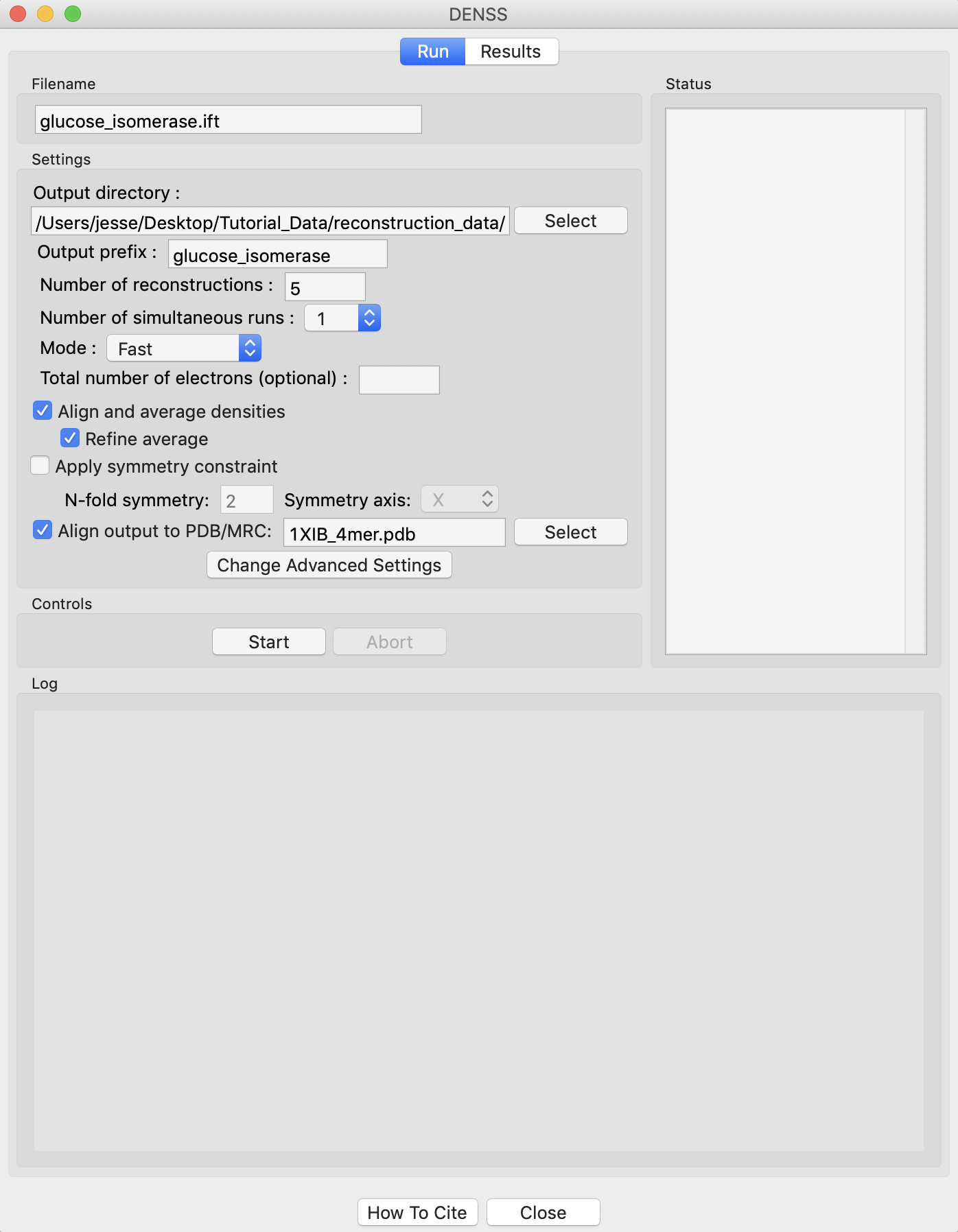
6. Click the “Start” button.

   • Note: The status panel will show you the overall status of the reconstructions. You can look at the detailed status of each run by clicking the appropriate tab in the log panel.

7. Note that by default the densities are aligned and averaged, including enantiomer filtering, and a refined density is created from the average.

8. Wait for all of the DENSS runs and averaging to finish. Depending on the speed of your computer this could take a bit.

9. Once the reconstructions are finished, the window should automatically switch to the results tab. If it doesn’t, click on the results tab.

   

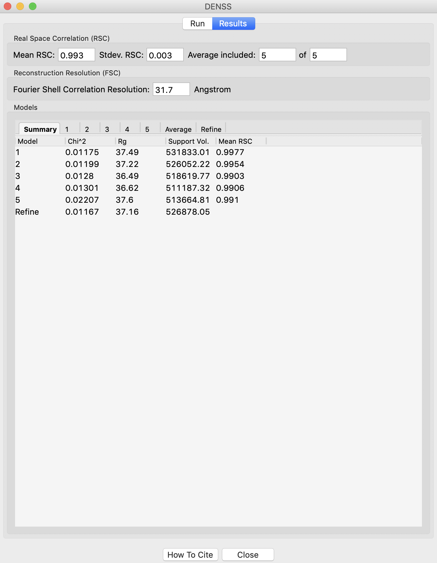
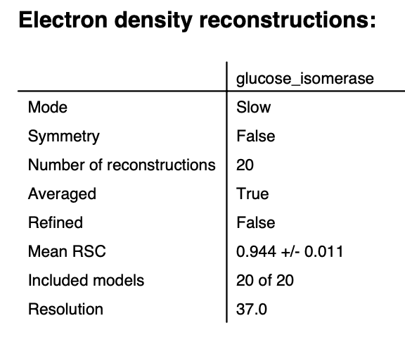
10. The results panel summarizes the results of the reconstruction runs. If you are using a .out file, then at the top of the panel there is the ambimeter evaluation of how ambiguous the reconstructions might be (see earlier tutorial section). If averaging was run there is an estimate of the reconstruction resolution based on the Fourier shell correlation. In the models section there are several tabs. The summary tab shows the chi^2, R_g, support volume, and RSC to the reference model. If any model was not included in the averaging it is highlighted in red.

    • Verify that the Rg is close to the expected value, and that the chi^2 and support volumes are relatively consistent between models.

    • Note: Above we show the results for 20 runs instead of the 5 in the tutorial.

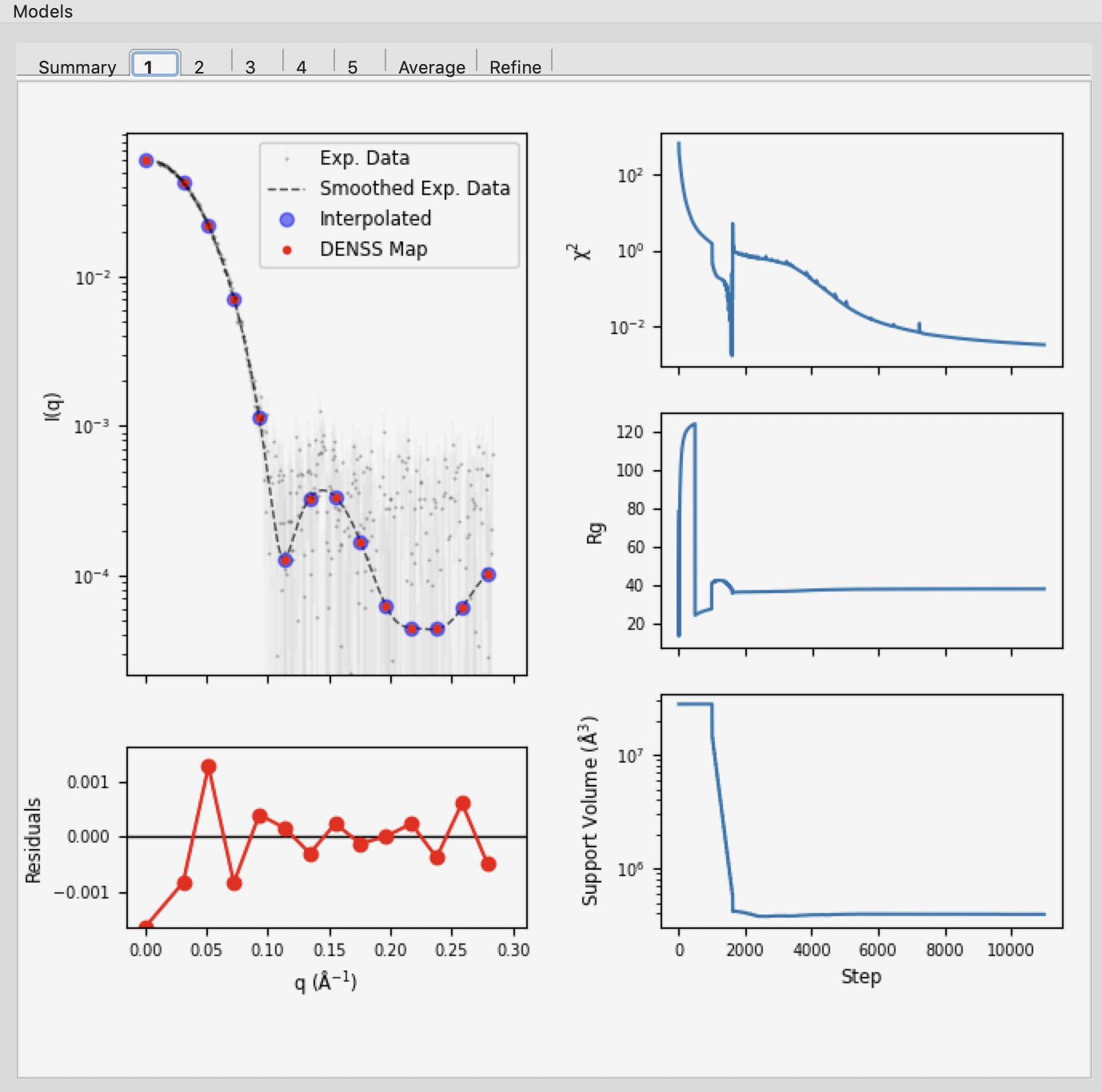
11. Individual model results are displayed in the numbered tabs. For each individual model there are plots of: the original data and the model data (scattering from density); the residual between the original data and the model data; and chi squared, R_g and support volume vs. refinement step.

    • Verify that the residual between the actual data and the model data is small.

    • Check that the chi squared, R_g, and support volume have all plateaued (converged) by the final steps.

    

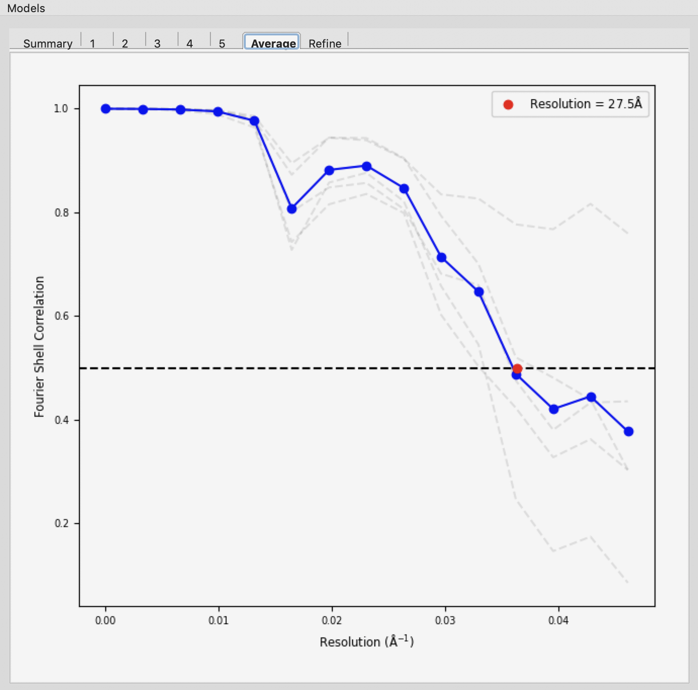
12. If the densities were averaged, the average tab will display the Fourier shell correlation vs. resolution.

    • Note: The reconstruction resolution is taken as the resolution in angstroms where the correlation first crosses 0.5.

    

13. The results summary shown in Summary tab is automatically saved as a <prefix>_denss_results.csv csv file, e.g. for this data as glucose_isomerase_denss_results.csv. All the plots shown on the individual model tabs are automatically saved as a multi-page pdf file with the same name.

14. Click the “Close” button when you are finished looking at the results and reconstructions.

15. The results from the individual DENSS runs are saved in the selected output folder as <prefix>_xx.mrc where xx corresponds to the run number: 01, 02, etc. For this tutorial that would be glucose_isomerase_01.mrc, glucose_isomerase_02.mrc, etc.

16. If averaging was done, final average density is saved in the selected output folder as <prefix>_aver.mrc. For this tutorial, that would be glucose_isomerase_aver.mrc.

17. If refinement was done, the final refined density is saved in the selected output folder as <prefix>_refine.mrc. For this tutorial that would be glucose_isomerase_refine.mrc.

18. If alignment to a reference model was done, the files aligned depend on what other processing was done.

    • If refinement was done, then there will be a single file named <prefix>_refine_aligned.mrc. For this tutorial, glucose_isomerase_refine_aligned.mrc.

    • If no refinement is done but averaging is done, then the averaged model is aligned. The associated filenames would be <prefix>_average_aligned.mrc. For this tutorial, glucose_isomerase_averaged_aligned.mrc.

    • If no refinement or averaging is done, then every calculated model is aligned. The associated filenames would be <prefix>_##_aligned.mrc where ## is the model number of a model. For this tutorial, that is glucose_isomerase_##_aligned.mrc.

19. You can save a summary table of the DENSS results with the pdf report that RAW can make. Close the DENSS window, right click on the glucose_isomerase.ift item in the IFT control panel and select “Save report”. Use the “Add DAMMIF/N results .csv” button to add the *glucose_isomerase_denss_results.csv to the report. Then click “Save Report” and save the pdf report. If you open the report you will see a summary of the run parameters and numerical results saved as a table.

    

Note: .mrc files can be opened in Chimera and pyMOL. For tips about how to visualize the density and align it with known structures see the appropriate sections here: http://www.tdgrant.com/denss/tips/.